Basic usage of tekkamaki

library(conflicted)
library(tekkamaki)
library(dplyr)
library(ggplot2)
palette_discrete = grDevices::palette.colors(palette = "Okabe-Ito")[-1]
theme_palette = ggplot2::theme(
  palette.colour.continuous = "viridis",
  palette.fill.continuous = "viridis",
  palette.colour.discrete = palette_discrete,
  palette.fill.discrete = palette_discrete
)

Run simulation:

set.seed(42)
result = tekka("-y80 -l3") |> print()

## # A tibble: 1 × 17
##   carrying_capacity fishing_coef fishing_mortality  last migration_matrices
##               <dbl> <list>       <list>            <int> <list>            
## 1              2000 <list [0]>   <dbl [84]>            3 <dbl [9 × 4 × 4]> 
## # ℹ 12 more variables: natural_mortality <list>, origin <int>, outdir <chr>,
## #   overdispersion <dbl>, recruitment <dbl>, sample_size_adult <list>,
## #   sample_size_juvenile <list>, seed <int>, weight_for_age <list>,
## #   years <int>, sample_family <list>, demography <list>

A result is a nested tibble with two columns: sample_family and demography:

sample_family = result$sample_family[[1L]] |> print()

## # A tibble: 6,712 × 6
##       id father_id mother_id birth_year location capture_year
##    <int>     <int>     <int>      <int>    <int>        <int>
##  1   133         0         0         -4       NA           NA
##  2   132       133       133          0       NA           NA
##  3   134       133       133          0       NA           NA
##  4   131       132       134          5       NA           NA
##  5   136       133       133          0       NA           NA
##  6   135       136       134          5       NA           NA
##  7   130       131       135         10       NA           NA
##  8   139       133       133          0       NA           NA
##  9   140       133       133          0       NA           NA
## 10   138       139       140          7       NA           NA
## # ℹ 6,702 more rows

demography = result$demography[[1L]] |> print()

## # A tibble: 6,599 × 5
##     year season location   age count
##    <int>  <int>    <int> <int> <int>
##  1     0      0        0     0  2000
##  2     0      1        0     0  1220
##  3     0      2        0     0   788
##  4     0      3        0     0   467
##  5     4      0        0     0  1057
##  6     4      0        0     4    19
##  7     4      1        0     0   682
##  8     4      1        0     4    14
##  9     4      2        0     0   425
## 10     4      2        0     4    14
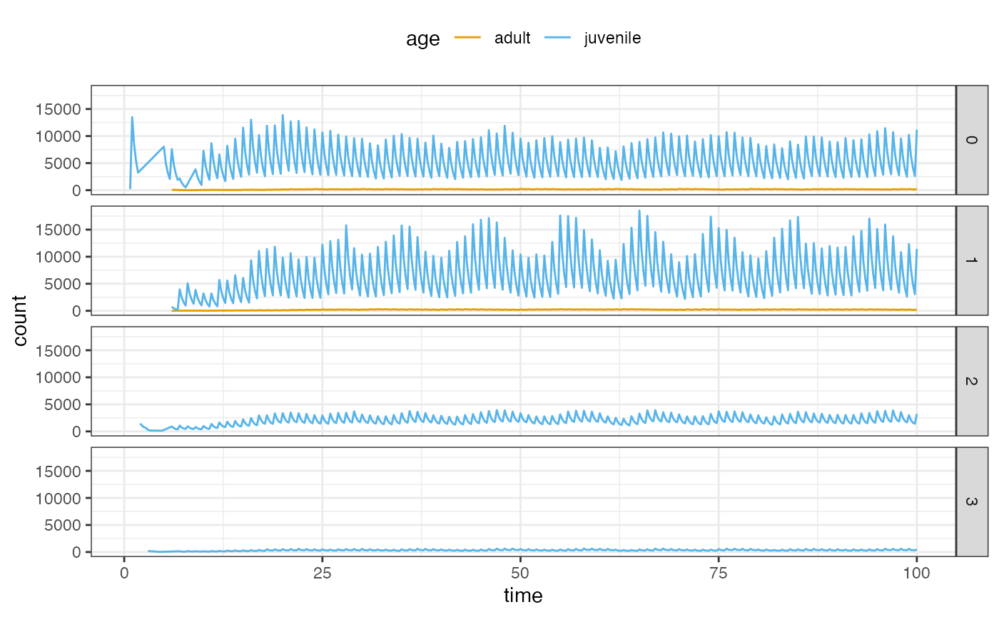
## # ℹ 6,589 more rows

Here is an example of visualizing demography:

df = demography |>
  dplyr::mutate(time = year + 0.25 * season) |>
  dplyr::mutate(age = ifelse(age >= 4, "adult", "juvenile")) |>
  dplyr::summarize(count = sum(count), .by = c(time, location, age)) |>
  tidyr::complete(time, location, age, fill = list(count = 0L))

ggplot(df) +
  aes(time, count) +
  geom_path(aes(colour = age, group = age)) +
  facet_grid(vars(location)) +
  theme_bw(base_size = 12) +
  theme_palette +
  theme(legend.position = "top")