統計モデリング実習 2022 TMDU

1. 導入、直線回帰
2. 確率分布、擬似乱数生成
3. 尤度、最尤推定
4. 一般化線形モデル (GLM)
5. 個体差、一般化線形混合モデル (GLMM)
6. ベイズの定理、事後分布、MCMC
7. StanでGLM
8. 階層ベイズモデル (HBM)

GLMMで登場した個体差を階層ベイズモデルで

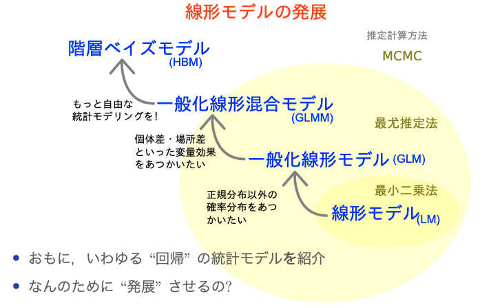
GLMMで登場した個体差を階層ベイズモデルで

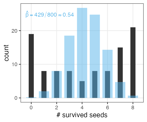
植物100個体から8個ずつ種子を取って植えたら全体で半分ちょい発芽。
親1個体あたりの生存数はn=8の二項分布になるはずだけど、
極端な値(全部死亡、全部生存)が多かった。個体差？

個体差をモデルに組み込みたい

各個体の生存率$p_i$をそのままパラメータにすると過剰適合。
「パラメータ数 ≥ サンプルサイズ」の“データ読み上げ”モデル。
i.e., この個体は4個生き残って生存率0.5だね。次の個体は2個体だから……

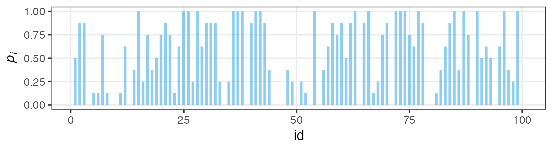
個体の生存能力をもっと少ないパラメータで表現できないか？

個体差をモデルに組み込みたい

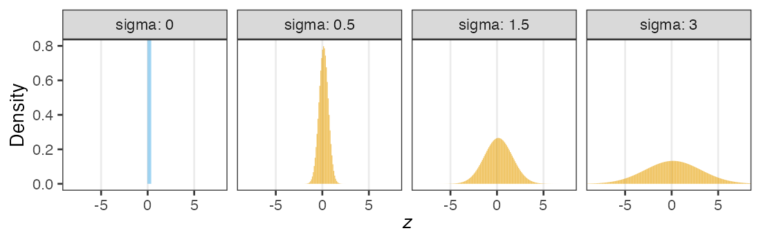
各個体の生存率$p_i$が能力値$z_i$のシグモイド関数で決まると仮定。
その能力値は全個体共通の正規分布に従うと仮定: $z_i \sim \mathcal{N}(\hat z, \sigma)$

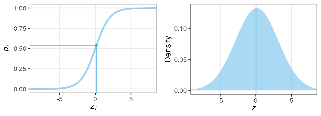
パラメータ2つで済む: 平均 $\hat z$, ばらつき $\sigma$ 。

前者は標本平均 $\hat p$ から求まるとして、後者どうする？

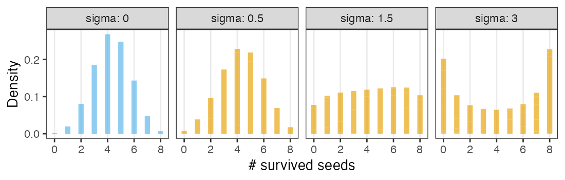
個体能力のばらつき $\sigma$ が大きいと両端が増える

普通の二項分布は個体差無し $\sigma = 0$ を仮定してるのと同じ。

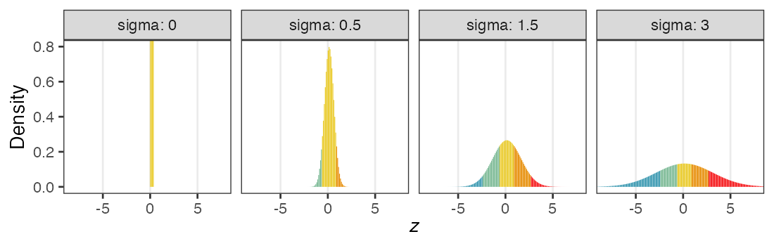
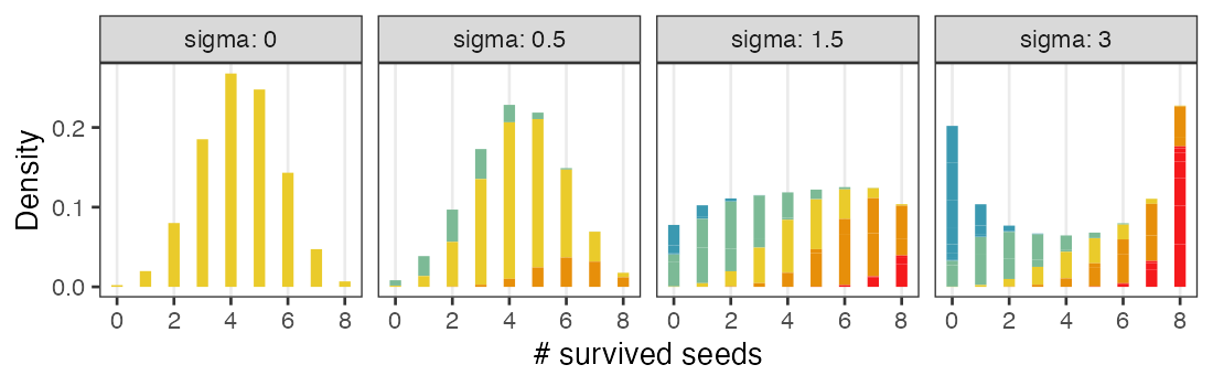
zの値で色分けしてみると想像しやすい

正規分布と二項分布の混ぜ合わせ……?

階層ベイズモデルのイメージ図

事前分布のパラメータに、さらに事前分布を設定するので階層ベイズ

さっきの図をStan言語で記述すると

10 とか 3 とか、エイヤっと決めてるやつが超パラメータ。

data {
  int<lower=0> N;
  array[N] int<lower=0> y;
}

parameters {
  real z_hat;           // mean ability
  real<lower=0> sigma;  // sd of r
  vector[N] r;          // individual difference
}

transformed parameters {
  vector[N] z = z_hat + r;
  vector[N] p = inv_logit(z);
}

model {
  y ~ binomial(8, p);
  z_hat ~ normal(0, 10);
  r ~ normal(0, sigma);
  sigma ~ student_t(3, 0, 1);
}

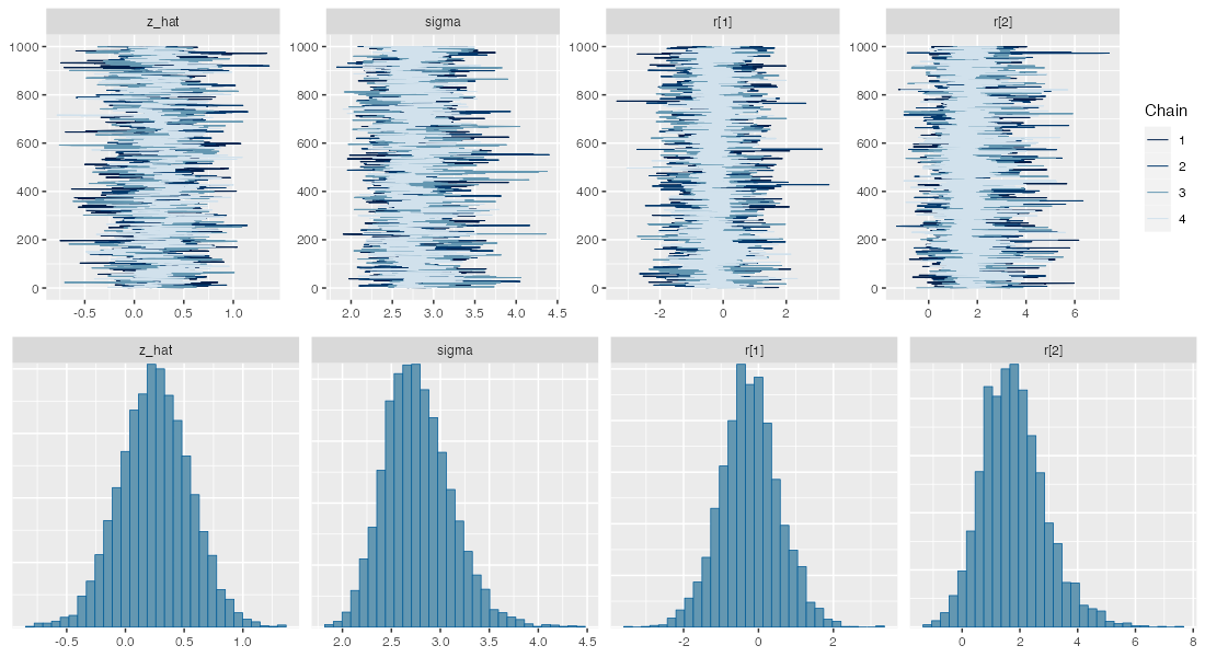
変量効果が入った推定結果

seeds_data = list(y = df_seeds_od$y, N = samplesize)
model = cmdstanr::cmdstan_model("stan/glmm.stan")
fit = model$sample(data = seeds_data, seed = 19937L, step_size = 0.1, refresh = 0)
draws = fit$draws(c("z_hat", "sigma", "r[1]", "r[2]"))

 variable    mean  median   sd  mad      q5     q95 rhat ess_bulk ess_tail
    lp__  -455.60 -455.30 9.34 9.25 -471.31 -441.11 1.00      784     1292
    z_hat    0.25    0.25 0.30 0.30   -0.24    0.74 1.00      777     1266
    sigma    2.77    2.75 0.34 0.33    2.26    3.37 1.00     1145     1581
    r[1]    -0.23   -0.25 0.78 0.74   -1.51    1.08 1.00     3484     2638
    r[2]     1.79    1.72 1.09 1.06    0.17    3.78 1.00     4776     2441
    r[3]     1.74    1.65 1.07 0.99    0.17    3.66 1.00     4304     2656
    r[4]    -3.73   -3.54 1.60 1.49   -6.69   -1.51 1.00     4847     2537
    r[5]    -2.20   -2.13 1.02 1.01   -4.00   -0.65 1.00     4411     2449
    r[6]    -2.17   -2.10 1.02 0.95   -4.00   -0.64 1.00     4336     2545
    r[7]     0.92    0.90 0.87 0.85   -0.45    2.40 1.00     4167     2377

 # showing 10 of 303 rows (change via 'max_rows' argument or 'cmdstanr_max_rows' option)

抜粋して作図。悪くない。

データ生成の真のパラメータ値は $\hat z = 0.5,~\sigma = 3.0$ だった。

🔰 階層ベイズモデルの練習問題: 種の数

100個体の植物から8つずつ種を取った、のデータでやってみよう。

sigmoid = function(x, gain = 1) {1 / (1 + exp(-gain * x))}
samplesize = 100L
df_seeds_od = tibble::tibble(
  z = rnorm(samplesize, 0.5, 3),
  p = sigmoid(z),
  y = rbinom(samplesize, 8L, p))

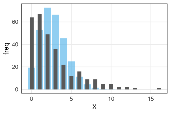
🔰 階層ベイズモデルの練習問題: ビール注文数

samplesize = 300L
lambda = 3
overdisp = 4
.n = lambda / (overdisp - 1)
.p = 1 / overdisp
df_beer_od = tibble::tibble(
  X = rnbinom(samplesize, size = .n, prob = .p)
)

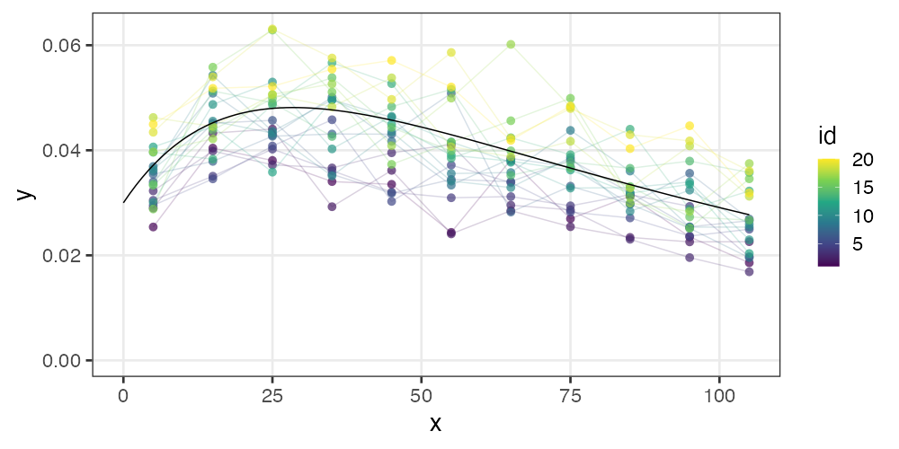
非線形回帰の例: データ

刺激強度xに対する応答強度yを20個体調査。
非対称なひと山。応答変数も説明変数も正の値。

非線形回帰の例: Stanコード

さっきの数式を model ブロックに書く。

data {
  int<lower=1> N;
  vector[N] x;
  vector[N] y;
  int id[N];
  int<lower=1> Ninds;
}

parameters {
  real<lower=0> a;
  real<lower=0> d;
  real<lower=0,upper=a> c;
  real<lower=0,upper=d> b;
  real shape;
  vector[Ninds] intercept;
}

model {
  vector[N] mu = a * exp(-b * x) - (a - c) * exp(-d * x) + intercept[id];
  y ~ gamma(shape, shape ./ mu);
  a ~ normal(0, 100);
  b ~ normal(0, 100);
  c ~ normal(0, 100);
  d ~ normal(0, 100);
  shape ~ normal(0, 100);
  intercept ~ normal(0, 0.005);
}

階層ベイズモデルのほかの応用先

• 時系列モデル (状態空間モデル)
• 空間構造のあるモデル (e.g., CARモデル)
• 欠損値の補完

ベイズ推定まとめ

• 条件付き確率 $\text{Prob}(B \mid A)$ の理解が大事。
  • 事後分布 $\propto$ 尤度 ⨉ 事前分布
  • 確信度合いをデータで更新していく。
• 推定結果は分布そのもの。
  • そこから点推定も区間推定も可能。
• 解析的に解けない問題は計算機に乱数を振らせて解く。
  • MCMCサンプル $\sim$ 解きにくい事後分布
  • 理論・技術の進歩が目覚ましい。

回帰分析ふりかえり

より柔軟にモデルを記述できるようになった。計算方法も変化。

全体まとめ

• 統計とは、データをうまくまとめ、それに基づいて推論するための手法。
• モデルには理解志向と応用志向があり、統計モデルは前者寄り。
  • どちらも多少は分かった上で使い分けたい。
  • どっちにしろ真の正しい何かではない。
• 確率分布とその背後にある確率過程の理解が重要。
  • 乱数生成→作図を繰り返してイメージを掴もう。
  • MCMCサンプリングも事後分布からの乱数生成。
• 本講義で「統計モデリングを完全に理解した」とは言えない。
  • 理論も実践もほとんど説明していない。
  • 本を読む準備ができた、くらいの気持ち？

参考文献

• データ解析のための統計モデリング入門 久保拓弥 2012
• StanとRでベイズ統計モデリング 松浦健太郎 2016
• RとStanではじめる ベイズ統計モデリングによるデータ分析入門 馬場真哉 2019
• データ分析のための数理モデル入門 江崎貴裕 2020
• 分析者のためのデータ解釈学入門 江崎貴裕 2020
• 統計学を哲学する 大塚淳 2020