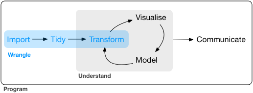
Hands-on R Lecture for Makino Lab
- Why do we use R?
- R basics
- Visualization with R
- Tidying and transforming data with R
- Statistical analysis with R
- File management with Git+GitHub
2019-10-16 生物棟大会議室
使える形にデータを整える
Happy families are all alike;
every unhappy family is unhappy in its own way
tidy datasets are all alike,
but every messy dataset is messy in its own way
- 出発点となるデータはさまざま
- laboratory notebook, field notebook、
- database, simulation…
- 解析や作図に使えるデータ形式はほぼ決まってる
ggplot(data, ...),glm(..., data, ...), …
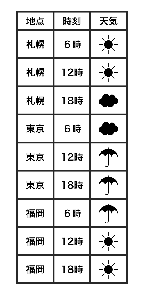
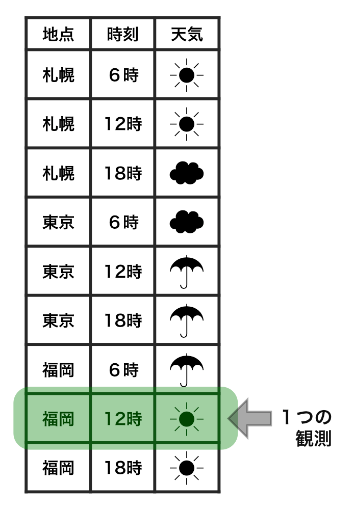
整然データ tidy data
- Each variable (変数) must have its own column (列).
- Each observation (観測) must have its own row (行).
- Each value must have its own cell.
print(diamonds)
      carat       cut color clarity depth table price     x     y     z
      <dbl>     <ord> <ord>   <ord> <dbl> <dbl> <int> <dbl> <dbl> <dbl>
    1  0.23     Ideal     E     SI2  61.5    55   326  3.95  3.98  2.43
    2  0.21   Premium     E     SI1  59.8    61   326  3.89  3.84  2.31
    3  0.23      Good     E     VS1  56.9    65   327  4.05  4.07  2.31
    4  0.29   Premium     I     VS2  62.4    58   334  4.20  4.23  2.63
   --
53937  0.72      Good     D     SI1  63.1    55  2757  5.69  5.75  3.61
53938  0.70 Very Good     D     SI1  62.8    60  2757  5.66  5.68  3.56
53939  0.86   Premium     H     SI2  61.0    58  2757  6.15  6.12  3.74
53940  0.75     Ideal     D     SI2  62.2    55  2757  5.83  5.87  3.64
https://r4ds.had.co.nz/tidy-data.html
https://speakerdeck.com/fnshr/zheng-ran-detatutenani
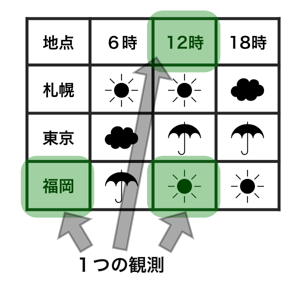
tidy data vs messy data
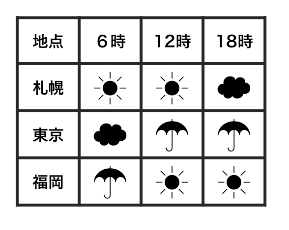
Each observation has its own row.
Each value has its own cell.
tidy data vs messy data
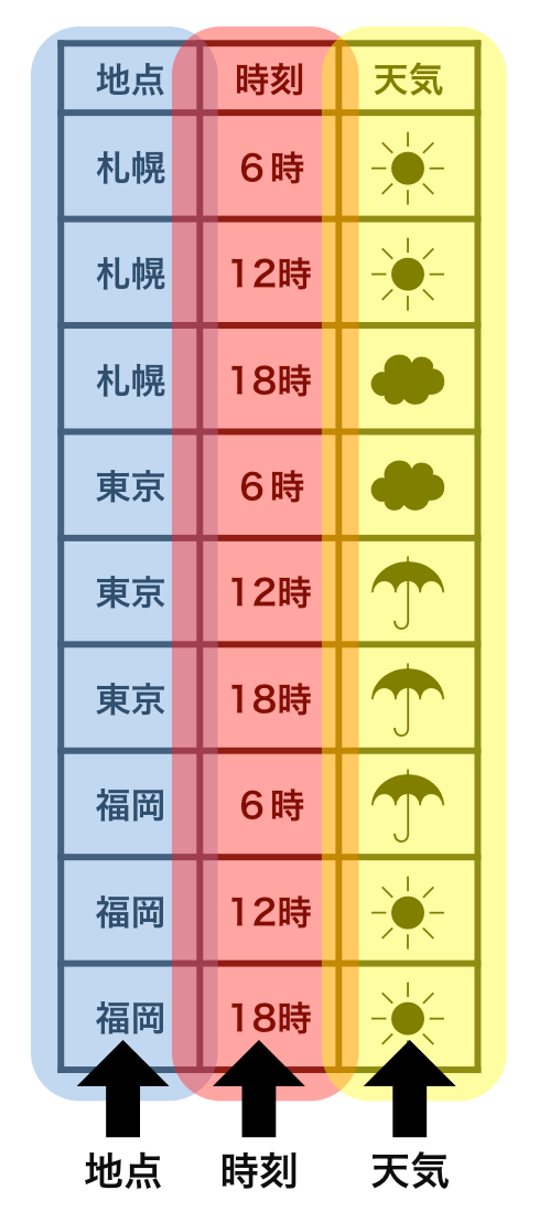
Each observation has its own row.
Each value has its own cell.
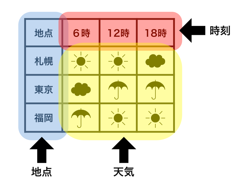
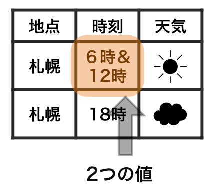
tidy data vs messy data
Each observation has its own row.
Each value has its own cell.
tidy data vs messy data
Each observation has its own row.
Each value has its own cell.
Today we learn data preparation
VADeaths
      Rural Male Rural Female Urban Male Urban Female
50-54       11.7          8.7       15.4          8.4
55-59       18.1         11.7       24.3         13.6
60-64       26.9         20.3       37.0         19.3
65-69       41.0         30.9       54.6         35.1
70-74       66.0         54.3       71.1         50.0
↓下ごしらえ
   lbound ubound region    sex death
    <int>  <int>  <chr>  <chr> <dbl>
 1     50     54  Rural   Male  11.7
 2     50     54  Rural Female   8.7
 3     50     54  Urban   Male  15.4
 4     50     54  Urban Female   8.4
--
17     70     74  Rural   Male  66.0
18     70     74  Rural Female  54.3
19     70     74  Urban   Male  71.1
20     70     74  Urban Female  50.0
tidyverseに便利な道具が揃ってる

Rでデータを上手に扱うためのパッケージ群
install.packages("tidyverse")
library(tidyverse)
# core packages are loaded
- 統一的な使い勝手
- シンプルな関数を繋げて使うデザイン
今回はそれらのごく一部をご紹介
dplyr — data.frameの高速処理担当

シンプルな関数がたくさん。
繋げて使う (piping)
- 抽出
filter(),select(),distinct(),sample_n()- 変更・追加
mutate(),rename()- 要約・集計
group_by(),summarize(),count()- ソート
arrange()- 結合
- 行方向:
bind_rows() - 列方向:
left_join(),inner_join(),full_join()
etc.
dplyrの基本的な使い方
小さな関数を繋げて使う。
result = diamonds %>%              # 生データから出発して
  select(carat, cut, price) %>%    # 列を抽出して
  filter(carat > 2) %>%            # 行を抽出して
  group_by(cut) %>%                # グループ化して
  summarize_all(mean) %>%          # それぞれ平均を計算
  print()                          # 表示してみる
        cut    carat    price
      <ord>    <dbl>    <dbl>
1      Fair 2.297692 11972.12
2      Good 2.139226 14628.99
3 Very Good 2.120232 15133.04
4   Premium 2.155707 14992.23
5     Ideal 2.147463 15589.13
What is %>% ?
Pipe operator (パイプ演算子) %>%
パイプの左側の変数を、右側の関数の第一引数にねじ込む:
# These are equivalent:
diamonds %>% filter(carat > 2)
filter(diamonds, carat > 2)
下ごしらえの流れ作業に便利:
diamonds %>% select(carat, price) %>% filter(carat > 2) %>% ...
#   data %>%  do_A()  %>%  do_B()  %>%  do_C()  %>% ...
[PRACTICE] Rewrite the following code without %>%:
seq_len(6) %>% sum()
[1] 21
letters %>% toupper() %>% head(3)
[1] "A" "B" "C"
[ANSWER]
sum(seq_len(6))
head(toupper(letters), 3)
If we don’t use pipe operator %>%
😐 Use temporary variables (一時変数):
tmp1 = select(diamonds, carat, cut, price)   # 列を抽出して
tmp2 = filter(tmp1, carat > 2)               # 行を抽出して
tmp3 = group_by(tmp2, cut)                   # グループ化して
result = summarize_all(tmp3, mean)           # それぞれ平均を計算
😐 Reuse the same variable:
result = select(diamonds, carat, cut, price) # 列を抽出して
result = filter(result, carat > 2)           # 行を抽出して
result = group_by(result, cut)               # グループ化して
result = summarize_all(result, mean)         # それぞれ平均を計算
Not too bad, but redundant.
If we don’t use pipe operator %>%
😫 Do it without temporary variables:
result = summarize_all(                # それぞれ平均を計算
    group_by(                            # グループ化して
      filter(                              # 行を抽出して
        select(diamonds, carat, cut, price), # 列を抽出して
        carat > 2),                        # 行を抽出して
      cut),                              # グループ化して
    mean)                              # それぞれ平均を計算
🤪 Unreadable:
result = summarize_all(group_by(filter(select(diamonds, carat, cut, price), carat > 2), cut), mean)
Very difficult to follow the logic.
Let’s use pipe operator %>%
😁 Easy to follow the logic:
result = diamonds %>%
  select(carat, cut, price) %>%    # 列を抽出して
  filter(carat > 2) %>%            # 行を抽出して
  group_by(cut) %>%                # グループ化して
  summarize_all(mean) %>%          # それぞれ平均を計算
  print()                          # 表示してみる
        cut    carat    price
      <ord>    <dbl>    <dbl>
1      Fair 2.297692 11972.12
2      Good 2.139226 14628.99
3 Very Good 2.120232 15133.04
4   Premium 2.155707 14992.23
5     Ideal 2.147463 15589.13
慣れるまではちょっと大変かも。無理して使わなくても大丈夫。
dplyr basics
Load the package, and view the data.
library(tidyverse)
print(diamonds)
View(diamonds)  # RStudio
      carat       cut color clarity depth table price     x     y     z
      <dbl>     <ord> <ord>   <ord> <dbl> <dbl> <int> <dbl> <dbl> <dbl>
    1  0.23     Ideal     E     SI2  61.5    55   326  3.95  3.98  2.43
    2  0.21   Premium     E     SI1  59.8    61   326  3.89  3.84  2.31
    3  0.23      Good     E     VS1  56.9    65   327  4.05  4.07  2.31
    4  0.29   Premium     I     VS2  62.4    58   334  4.20  4.23  2.63
   --
53937  0.72      Good     D     SI1  63.1    55  2757  5.69  5.75  3.61
53938  0.70 Very Good     D     SI1  62.8    60  2757  5.66  5.68  3.56
53939  0.86   Premium     H     SI2  61.0    58  2757  6.15  6.12  3.74
53940  0.75     Ideal     D     SI2  62.2    55  2757  5.83  5.87  3.64
dplyr basics: select()
Select columns (列) by names.
result = diamonds %>%
  select(carat, cut, price) %>%
  print()
      carat       cut price
      <dbl>     <ord> <int>
    1  0.23     Ideal   326
    2  0.21   Premium   326
    3  0.23      Good   327
    4  0.29   Premium   334
   --
53937  0.72      Good  2757
53938  0.70 Very Good  2757
53939  0.86   Premium  2757
53940  0.75     Ideal  2757
dplyr basics: select()
Select columns (列) by numbers.
result = diamonds %>%
  select(1, 2, 7) %>%
  print()
      carat       cut price
      <dbl>     <ord> <int>
    1  0.23     Ideal   326
    2  0.21   Premium   326
    3  0.23      Good   327
    4  0.29   Premium   334
   --
53937  0.72      Good  2757
53938  0.70 Very Good  2757
53939  0.86   Premium  2757
53940  0.75     Ideal  2757
dplyr basics: select()
Select columns (列) by negative match.
result = diamonds %>%
  select(-carat, -cut, -price) %>%
  print()
      color clarity depth table     x     y     z
      <ord>   <ord> <dbl> <dbl> <dbl> <dbl> <dbl>
    1     E     SI2  61.5    55  3.95  3.98  2.43
    2     E     SI1  59.8    61  3.89  3.84  2.31
    3     E     VS1  56.9    65  4.05  4.07  2.31
    4     I     VS2  62.4    58  4.20  4.23  2.63
   --
53937     D     SI1  63.1    55  5.69  5.75  3.61
53938     D     SI1  62.8    60  5.66  5.68  3.56
53939     H     SI2  61.0    58  6.15  6.12  3.74
53940     D     SI2  62.2    55  5.83  5.87  3.64
dplyr basics: select()
Select columns (列) by partial match.
result = diamonds %>%
  select(starts_with("c")) %>%
  print()
      carat       cut color clarity
      <dbl>     <ord> <ord>   <ord>
    1  0.23     Ideal     E     SI2
    2  0.21   Premium     E     SI1
    3  0.23      Good     E     VS1
    4  0.29   Premium     I     VS2
   --
53937  0.72      Good     D     SI1
53938  0.70 Very Good     D     SI1
53939  0.86   Premium     H     SI2
53940  0.75     Ideal     D     SI2
See tidyselect helpers for more details.
dplyr basics: filter()
Filter rows (行) by exact match.
result = diamonds %>%
  filter(cut == "Ideal") %>%
  print()
      carat   cut color clarity depth table price     x     y     z
      <dbl> <ord> <ord>   <ord> <dbl> <dbl> <int> <dbl> <dbl> <dbl>
    1  0.23 Ideal     E     SI2  61.5    55   326  3.95  3.98  2.43
    2  0.23 Ideal     J     VS1  62.8    56   340  3.93  3.90  2.46
    3  0.31 Ideal     J     SI2  62.2    54   344  4.35  4.37  2.71
    4  0.30 Ideal     I     SI2  62.0    54   348  4.31  4.34  2.68
   --
21548  0.71 Ideal     E     SI1  61.9    56  2756  5.71  5.73  3.54
21549  0.71 Ideal     G     VS1  61.4    56  2756  5.76  5.73  3.53
21550  0.72 Ideal     D     SI1  60.8    57  2757  5.75  5.76  3.50
21551  0.75 Ideal     D     SI2  62.2    55  2757  5.83  5.87  3.64
dplyr basics: filter()
Filter rows (行) by group membership.
result = diamonds %>%
  filter(cut %in% c("Ideal", "Good")) %>%
  print()
      carat   cut color clarity depth table price     x     y     z
      <dbl> <ord> <ord>   <ord> <dbl> <dbl> <int> <dbl> <dbl> <dbl>
    1  0.23 Ideal     E     SI2  61.5    55   326  3.95  3.98  2.43
    2  0.23  Good     E     VS1  56.9    65   327  4.05  4.07  2.31
    3  0.31  Good     J     SI2  63.3    58   335  4.34  4.35  2.75
    4  0.30  Good     J     SI1  64.0    55   339  4.25  4.28  2.73
   --
26454  0.71 Ideal     G     VS1  61.4    56  2756  5.76  5.73  3.53
26455  0.72 Ideal     D     SI1  60.8    57  2757  5.75  5.76  3.50
26456  0.72  Good     D     SI1  63.1    55  2757  5.69  5.75  3.61
26457  0.75 Ideal     D     SI2  62.2    55  2757  5.83  5.87  3.64
dplyr basics: filter()
Filter rows (行) with unequal sign.
result = diamonds %>%
  filter(price >= 1000) %>%
  print()
      carat       cut color clarity depth table price     x     y     z
      <dbl>     <ord> <ord>   <ord> <dbl> <dbl> <int> <dbl> <dbl> <dbl>
    1  0.70     Ideal     E     SI1  62.5    57  2757  5.70  5.72  3.57
    2  0.86      Fair     E     SI2  55.1    69  2757  6.45  6.33  3.52
    3  0.70     Ideal     G     VS2  61.6    56  2757  5.70  5.67  3.50
    4  0.71 Very Good     E     VS2  62.4    57  2759  5.68  5.73  3.56
   --
39438  0.72      Good     D     SI1  63.1    55  2757  5.69  5.75  3.61
39439  0.70 Very Good     D     SI1  62.8    60  2757  5.66  5.68  3.56
39440  0.86   Premium     H     SI2  61.0    58  2757  6.15  6.12  3.74
39441  0.75     Ideal     D     SI2  62.2    55  2757  5.83  5.87  3.64
dplyr basics: filter()
Filter rows (行) by multiple conditions (AND).
result = diamonds %>%
  filter(carat > 2 & price < 14000) %>%
  print()
    carat       cut color clarity depth table price     x     y     z
    <dbl>     <ord> <ord>   <ord> <dbl> <dbl> <int> <dbl> <dbl> <dbl>
  1  2.06   Premium     J      I1  61.2    58  5203  8.10  8.07  4.95
  2  2.14      Fair     J      I1  69.4    57  5405  7.74  7.70  5.36
  3  2.15      Fair     J      I1  65.5    57  5430  8.01  7.95  5.23
  4  2.22      Fair     J      I1  66.7    56  5607  8.04  8.02  5.36
 --
641  2.07   Premium     H     SI1  62.7    58 13993  8.14  8.09  5.09
642  2.07      Good     I     SI1  63.6    58 13993  8.09  7.99  5.11
643  2.13 Very Good     J     SI1  62.8    58 13996  8.13  8.17  5.12
644  2.11   Premium     J     SI1  62.4    58 13996  8.27  8.17  5.13
dplyr basics: filter()
Filter rows (行) by multiple conditions (OR).
result = diamonds %>%
  filter(carat > 2 | price < 14000) %>%
  print()
      carat       cut color clarity depth table price     x     y     z
      <dbl>     <ord> <ord>   <ord> <dbl> <dbl> <int> <dbl> <dbl> <dbl>
    1  0.23     Ideal     E     SI2  61.5    55   326  3.95  3.98  2.43
    2  0.21   Premium     E     SI1  59.8    61   326  3.89  3.84  2.31
    3  0.23      Good     E     VS1  56.9    65   327  4.05  4.07  2.31
    4  0.29   Premium     I     VS2  62.4    58   334  4.20  4.23  2.63
   --
53023  0.72      Good     D     SI1  63.1    55  2757  5.69  5.75  3.61
53024  0.70 Very Good     D     SI1  62.8    60  2757  5.66  5.68  3.56
53025  0.86   Premium     H     SI2  61.0    58  2757  6.15  6.12  3.74
53026  0.75     Ideal     D     SI2  62.2    55  2757  5.83  5.87  3.64
dplyr basics: mutate()
Create new columns or modify existing columns.
result = diamonds %>%
  mutate(ratio = price / carat,
         price = price * 108.36) %>%
  print()
      carat       cut color clarity depth table     price     x     y     z    ratio
      <dbl>     <ord> <ord>   <ord> <dbl> <dbl>     <dbl> <dbl> <dbl> <dbl>    <dbl>
    1  0.23     Ideal     E     SI2  61.5    55  35325.36  3.95  3.98  2.43 1417.391
    2  0.21   Premium     E     SI1  59.8    61  35325.36  3.89  3.84  2.31 1552.381
    3  0.23      Good     E     VS1  56.9    65  35433.72  4.05  4.07  2.31 1421.739
    4  0.29   Premium     I     VS2  62.4    58  36192.24  4.20  4.23  2.63 1151.724
   --
53937  0.72      Good     D     SI1  63.1    55 298748.52  5.69  5.75  3.61 3829.167
53938  0.70 Very Good     D     SI1  62.8    60 298748.52  5.66  5.68  3.56 3938.571
53939  0.86   Premium     H     SI2  61.0    58 298748.52  6.15  6.12  3.74 3205.814
53940  0.75     Ideal     D     SI2  62.2    55 298748.52  5.83  5.87  3.64 3676.000
dplyr basics: summarize()
Summarize column values.
result = diamonds %>%
  summarize(mean(price), max(carat)) %>%
  print()
  mean(price) max(carat)
        <dbl>      <dbl>
1      3932.8       5.01
Use min(), max(), mean(), median(), var(), sd(), etc.
dplyr basics: summarize()
Summarize column values by groups.
result = diamonds %>%
  group_by(cut) %>%
  summarize(avg_price = mean(price),
            max_carat = max(carat)) %>%
  print()
        cut avg_price max_carat
      <ord>     <dbl>     <dbl>
1      Fair  4358.758      5.01
2      Good  3928.864      3.01
3 Very Good  3981.760      4.00
4   Premium  4584.258      4.01
5     Ideal  3457.542      3.50
dplyr basics: arrange()
Sort rows. Use desc() for reversed order.
result = diamonds %>%
  arrange(color, desc(carat)) %>%  # 色の昇順。色が同じなら大きさ降順
  print()
      carat       cut color clarity depth table price     x     y     z
      <dbl>     <ord> <ord>   <ord> <dbl> <dbl> <int> <dbl> <dbl> <dbl>
    1  3.40      Fair     D      I1  66.8    52 15964  9.42  9.34  6.27
    2  2.75     Ideal     D      I1  60.9    57 13156  9.04  8.98  5.49
    3  2.58 Very Good     D     SI2  58.9    63 14749  9.08  9.01  5.33
    4  2.57   Premium     D     SI2  58.9    58 17924  8.99  8.94  5.28
   --
53937  0.27 Very Good     J    VVS2  60.8    57   443  4.16  4.20  2.54
53938  0.24 Very Good     J    VVS2  62.8    57   336  3.94  3.96  2.48
53939  0.24     Ideal     J    VVS2  62.8    57   432  3.96  3.94  2.48
53940  0.23     Ideal     J     VS1  62.8    56   340  3.93  3.90  2.46
dplyr basics: *_join()
Combine two tables depending on column values.
band_members %>% inner_join(band_instruments, by = "name")
   name    band  plays
  <chr>   <chr>  <chr>
1  John Beatles guitar
2  Paul Beatles   bass
band_members %>% left_join(band_instruments, by = "name")
   name    band  plays
  <chr>   <chr>  <chr>
1  Mick  Stones   <NA>
2  John Beatles guitar
3  Paul Beatles   bass
band_members %>% full_join(band_instruments, by = "name")
   name    band  plays
  <chr>   <chr>  <chr>
1  Mick  Stones   <NA>
2  John Beatles guitar
3  Paul Beatles   bass
4 Keith    <NA> guitar
tidyr — data.frameの変形・整形担当

- 横長から縦長に
pivot_longer()- 縦長から横長に
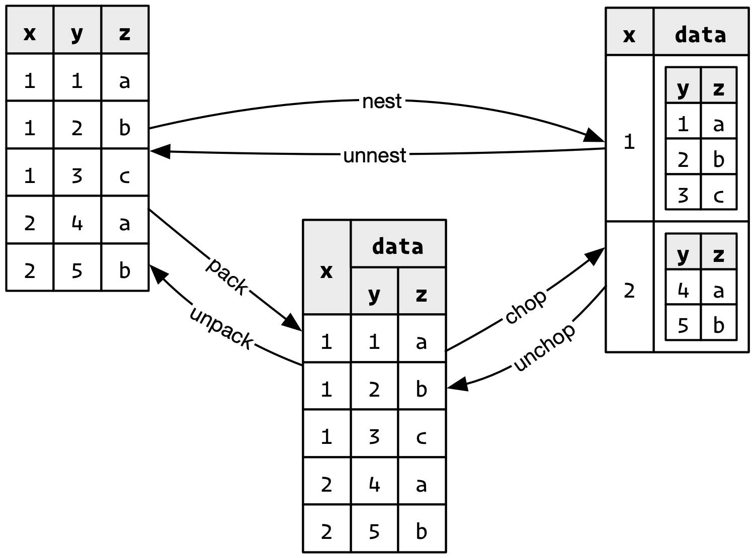
pivot_wider()- 入れ子構造をつくる、解消する
nest(),unnest()- 1列を複数の列に分離
separate()
etc.
tidyr::pivot_longer() 横長から縦長に
複数列にまたがる値を1列にする(ここではvalue)。
そのラベルも合わせて移動(ここではname)。
iris_long = iris %>% head(2L) %>%     # 最初の2行だけ
  rownames_to_column("id") %>%        # ID列を追加
  print() %>%                         # 途中経過を表示
  pivot_longer(c(-id, -Species), names_to = "name", values_to = "value") %>%
  print()                             # id, Species以外の値を移動
     id Sepal.Length Sepal.Width Petal.Length Petal.Width Species
  <chr>        <dbl>       <dbl>        <dbl>       <dbl>   <fct>
1     1          5.1         3.5          1.4         0.2  setosa
2     2          4.9         3.0          1.4         0.2  setosa
     id Species         name value
  <chr>   <fct>        <chr> <dbl>
1     1  setosa Sepal.Length   5.1
2     1  setosa  Sepal.Width   3.5
3     1  setosa Petal.Length   1.4
4     1  setosa  Petal.Width   0.2
5     2  setosa Sepal.Length   4.9
6     2  setosa  Sepal.Width   3.0
7     2  setosa Petal.Length   1.4
8     2  setosa  Petal.Width   0.2
tidyr::pivot_wider() 縦長から横長に
1列に収まっていた値(value)を複数列の行列に変換。
そのラベル(name)を列の名前にする。
iris_long %>% print() %>%              # さっきlong-formatにしたやつ
  pivot_wider(names_from = name, values_from = value)   # 横長に戻す
     id Species         name value
  <chr>   <fct>        <chr> <dbl>
1     1  setosa Sepal.Length   5.1
2     1  setosa  Sepal.Width   3.5
3     1  setosa Petal.Length   1.4
4     1  setosa  Petal.Width   0.2
5     2  setosa Sepal.Length   4.9
6     2  setosa  Sepal.Width   3.0
7     2  setosa Petal.Length   1.4
8     2  setosa  Petal.Width   0.2
     id Species Sepal.Length Sepal.Width Petal.Length Petal.Width
  <chr>   <fct>        <dbl>       <dbl>        <dbl>       <dbl>
1     1  setosa          5.1         3.5          1.4         0.2
2     2  setosa          4.9         3.0          1.4         0.2
tidyr::separate() 列を分離
iris_long %>% print() %>%
  separate(name, c("part", "measure")) # 列を分離
     id Species         name value
  <chr>   <fct>        <chr> <dbl>
1     1  setosa Sepal.Length   5.1
2     1  setosa  Sepal.Width   3.5
3     1  setosa Petal.Length   1.4
4     1  setosa  Petal.Width   0.2
5     2  setosa Sepal.Length   4.9
6     2  setosa  Sepal.Width   3.0
7     2  setosa Petal.Length   1.4
8     2  setosa  Petal.Width   0.2
     id Species  part measure value
  <chr>   <fct> <chr>   <chr> <dbl>
1     1  setosa Sepal  Length   5.1
2     1  setosa Sepal   Width   3.5
3     1  setosa Petal  Length   1.4
4     1  setosa Petal   Width   0.2
5     2  setosa Sepal  Length   4.9
6     2  setosa Sepal   Width   3.0
7     2  setosa Petal  Length   1.4
8     2  setosa Petal   Width   0.2
tidyr::nest() 入れ子にする
グループ毎にdata.frameを区切ってlist型の列に入れる。
tidyr::nest() 入れ子にする
グループ毎にdata.frameを区切ってlist型の列に入れる。
iris_nested = iris %>%
  as_tibble() %>%
  nest(data = -Species) %>% print()
     Species              data
       <fct>            <list>
1     setosa <tbl_df [50 x 4]>
2 versicolor <tbl_df [50 x 4]>
3  virginica <tbl_df [50 x 4]>
iris_nested$data[[1L]]
   Sepal.Length Sepal.Width Petal.Length Petal.Width
          <dbl>       <dbl>        <dbl>       <dbl>
 1          5.1         3.5          1.4         0.2
 2          4.9         3.0          1.4         0.2
 3          4.7         3.2          1.3         0.2
 4          4.6         3.1          1.5         0.2
--
47          5.1         3.8          1.6         0.2
48          4.6         3.2          1.4         0.2
49          5.3         3.7          1.5         0.2
50          5.0         3.3          1.4         0.2
purrr
listやループの処理担当。
map(),walk()map_int(),map_dbl(),map_chr()map_dfr()pmap(),map2()flatten()- etc.
標準Rの lapply(), sapply(), vapply(), unlist() などの代わりに
purrr::map(): リストの各要素に関数を適用
v = c(1, 2, 3)      # 長さ3のベクトル
v + 10              # それぞれに+10
[1] 11 12 13
plus_ten = function(x) {x + 10}  # +10する関数
purrr::map(v, plus_ten)          # それぞれに適用
[[1]]
[1] 11

[[2]]
[1] 12

[[3]]
[1] 13
この例ではあまり嬉しくないけど、使いどころは結構ある
Read multiple files in a directory
r-training-2019/       # プロジェクトの最上階
├── data/              # データを置くディレクトリ
│   ├── cheetah.tsv    # 同じ形のデータ
│   ├── giraffe.tsv
│   └── zebra.tsv
├─
# Get the file list: "data/cheetah.tsv", ...
files = fs::dir_ls("data", glob = "*.tsv")

# Read and combine
purrr::map_dfr(files, readr::read_tsv)

# It is equivalent to
purrr::map(files, readr::read_tsv) %>%
  dplyr::bind_rows()
Example: VADeaths
as.data.frame(VADeaths)                  # data.frameに変換
                                         # 行名を列に
                                         # 縦長に変形したい
      Rural Male Rural Female Urban Male Urban Female
50-54       11.7          8.7       15.4          8.4
55-59       18.1         11.7       24.3         13.6
60-64       26.9         20.3       37.0         19.3
65-69       41.0         30.9       54.6         35.1
70-74       66.0         54.3       71.1         50.0
Example: VADeaths
as.data.frame(VADeaths) %>%              # data.frameに変換
  tibble::rownames_to_column("age")      # 行名を列に
                                         # 縦長に変形したい
    age Rural Male Rural Female Urban Male Urban Female
1 50-54       11.7          8.7       15.4          8.4
2 55-59       18.1         11.7       24.3         13.6
3 60-64       26.9         20.3       37.0         19.3
4 65-69       41.0         30.9       54.6         35.1
5 70-74       66.0         54.3       71.1         50.0
Example: VADeaths
as.data.frame(VADeaths) %>%              # data.frameに変換
  tibble::rownames_to_column("age") %>%  # 行名を列に
  pivot_longer(-age)                     # age以外を移動して縦長化
                                         # 新しいname列を分割
     age         name value
   <chr>        <chr> <dbl>
 1 50-54   Rural Male  11.7
 2 50-54 Rural Female   8.7
 3 50-54   Urban Male  15.4
 4 50-54 Urban Female   8.4
--
17 70-74   Rural Male  66.0
18 70-74 Rural Female  54.3
19 70-74   Urban Male  71.1
20 70-74 Urban Female  50.0
Example: VADeaths
as.data.frame(VADeaths) %>%              # data.frameに変換
  tibble::rownames_to_column("age") %>%  # 行名を列に
  pivot_longer(-age) %>%                 # age以外を移動して縦長化
  separate(name, c("region", "sex"))     # 新しいname列を分割
     age region    sex value
   <chr>  <chr>  <chr> <dbl>
 1 50-54  Rural   Male  11.7
 2 50-54  Rural Female   8.7
 3 50-54  Urban   Male  15.4
 4 50-54  Urban Female   8.4
--
17 70-74  Rural   Male  66.0
18 70-74  Rural Female  54.3
19 70-74  Urban   Male  71.1
20 70-74  Urban Female  50.0
Example: VADeaths
va_deaths = as.data.frame(VADeaths) %>%  # data.frameに変換
  tibble::rownames_to_column("age") %>%  # 行名を列に
  pivot_longer(-age) %>%                 # age以外を移動して縦長化
  separate(name, c("region", "sex")) %>% # 新しいname列を分割
  separate(age, c("lbound", "ubound"), "-", convert = TRUE) %>%
  print()                                # 下限と上限を分離
   lbound ubound region    sex value
    <int>  <int>  <chr>  <chr> <dbl>
 1     50     54  Rural   Male  11.7
 2     50     54  Rural Female   8.7
 3     50     54  Urban   Male  15.4
 4     50     54  Urban Female   8.4
--
17     70     74  Rural   Male  66.0
18     70     74  Rural Female  54.3
19     70     74  Urban   Male  71.1
20     70     74  Urban Female  50.0
Example: VADeaths 別解
va_deaths = as.data.frame(VADeaths) %>%  # data.frameに変換
  tibble::rownames_to_column("age") %>%  # 行名を列に
  tidyr::pivot_longer(                   # 縦長に変形したい
    -age,                                # age以外の列に入ってる値を移動
    names_to = c("region", "sex"),       # 元の列名を2つに分離
    names_sep = " ",                     # スペースで切る
    values_to = "death") %>%             # 値の行き先の列名
  tidyr::separate(age, c("lbound", "ubound"), "-", convert = TRUE) %>%
  print()                                # 下限と上限を分離
   lbound ubound region    sex death
    <int>  <int>  <chr>  <chr> <dbl>
 1     50     54  Rural   Male  11.7
 2     50     54  Rural Female   8.7
 3     50     54  Urban   Male  15.4
 4     50     54  Urban Female   8.4
--
17     70     74  Rural   Male  66.0
18     70     74  Rural Female  54.3
19     70     74  Urban   Male  71.1
20     70     74  Urban Female  50.0
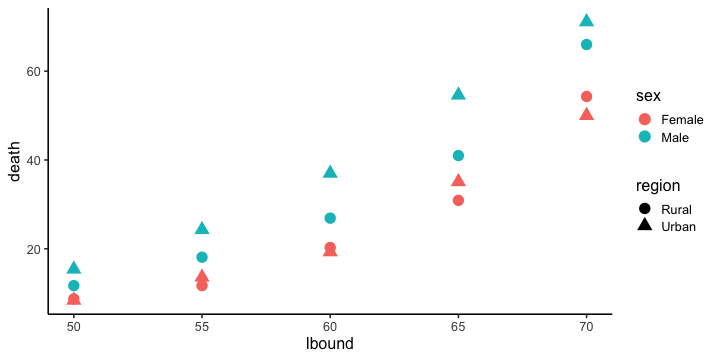
Example: VADeaths
va_deaths %>%
  ggplot(aes(lbound, death)) +
  geom_point(aes(color = sex, shape = region), size = 5) +
  theme_classic(base_size = 16)
Visualize and summarize anscombe
4組のx-yは、平均・分散・相関係数がほぼ同じ?
anscombe %>%
  rowid_to_column("id")              # IDをつけておく
                                     # x y で始まる列の値を移して縦長に
      id    x1    x2    x3    x4    y1    y2    y3    y4
   <int> <dbl> <dbl> <dbl> <dbl> <dbl> <dbl> <dbl> <dbl>
 1     1    10    10    10     8  8.04  9.14  7.46  6.58
 2     2     8     8     8     8  6.95  8.14  6.77  5.76
 3     3    13    13    13     8  7.58  8.74 12.74  7.71
 4     4     9     9     9     8  8.81  8.77  7.11  8.84
--
 8     8     4     4     4    19  4.26  3.10  5.39 12.50
 9     9    12    12    12     8 10.84  9.13  8.15  5.56
10    10     7     7     7     8  4.82  7.26  6.42  7.91
11    11     5     5     5     8  5.68  4.74  5.73  6.89
ggplot does not accept this format. Let’s transformt it.
Visualize and summarize anscombe
4組のx-yは、平均・分散・相関係数がほぼ同じ?
anscombe %>%
  rowid_to_column("id") %>%          # IDをつけておく
  pivot_longer(matches("^x|y"))      # x y で始まる列の値を移して縦長に

                                     # name列を分割
      id  name value
   <int> <chr> <dbl>
 1     1    x1 10.00
 2     1    x2 10.00
 3     1    x3 10.00
 4     1    x4  8.00
--
85    11    y1  5.68
86    11    y2  4.74
87    11    y3  5.73
88    11    y4  6.89
Visualize and summarize anscombe
4組のx-yは、平均・分散・相関係数がほぼ同じ?
anscombe %>%
  rowid_to_column("id") %>%          # IDをつけておく
  pivot_longer(matches("^x|y")) %>%  # x y で始まる列の値を移して縦長に
  separate(name, c("axis", "group"), 1L, convert = TRUE)
                                     # name列を分割
      id  axis group value
   <int> <chr> <int> <dbl>
 1     1     x     1 10.00
 2     1     x     2 10.00
 3     1     x     3 10.00
 4     1     x     4  8.00
--
85    11     y     1  5.68
86    11     y     2  4.74
87    11     y     3  5.73
88    11     y     4  6.89
Visualize and summarize anscombe
4組のx-yは、平均・分散・相関係数がほぼ同じ?
tidy_anscombe = anscombe %>%
  rowid_to_column("id") %>%          # IDをつけておく
  pivot_longer(matches("^x|y")) %>%  # x y で始まる列の値を移して縦長に
  separate(name, c("axis", "group"), 1L, convert = TRUE) %>%
                                     # name列を分割
  pivot_wider(names_from = axis, values_from = value) %>%
                                     # axis列内の x y を列にして横長化
  dplyr::arrange(group) %>%          # グループごとに並べる
  print()                            # ggplotしたい形!
      id group     x     y
   <int> <int> <dbl> <dbl>
 1     1     1    10  8.04
 2     2     1     8  6.95
 3     3     1    13  7.58
 4     4     1     9  8.81
--
41     8     4    19 12.50
42     9     4     8  5.56
43    10     4     8  7.91
44    11     4     8  6.89
Visualize and summarize anscombe 別解
4組のx-yは、平均・分散・相関係数がほぼ同じ?
tidy_anscombe = anscombe %>%
  tidyr::pivot_longer(                # 縦長に変形したい
    everything(),                     # すべての列について
    names_to = c(".value", "group"),  # 新しい列名
    names_sep = 1L) %>%               # 切る位置
  dplyr::mutate(group = as.integer(group)) %>% # 型変換
  dplyr::arrange(group) %>%           # グループごとに並べる
  print()                             # ggplotしたい形!
   group     x     y
   <int> <dbl> <dbl>
 1     1    10  8.04
 2     1     8  6.95
 3     1    13  7.58
 4     1     9  8.81
--
41     4    19 12.50
42     4     8  5.56
43     4     8  7.91
44     4     8  6.89
Visualize and summarize anscombe
4組のx-yは、平均・分散・相関係数がほぼ同じ?
ggplot(tidy_anscombe, aes(x, y)) +
  geom_point(size = 3) +
  stat_smooth(method = lm, formula = y ~ x, se = FALSE, fullrange = TRUE) +
  facet_wrap(~ group, nrow = 1L)

Visualize and summarize anscombe
4組のx-yは、平均・分散・相関係数がほぼ同じ?
tidy_anscombe %>%
  dplyr::group_by(group) %>%   # group列でグループ化して
  dplyr::summarize(            # x, y列を使ってsummarize
    mean_x = mean(x),
    mean_y = mean(y),
    sd_x = sd(x),
    sd_y = sd(y),
    cor_xy = cor(x, y)
  )
  group mean_x   mean_y     sd_x     sd_y    cor_xy
  <int>  <dbl>    <dbl>    <dbl>    <dbl>     <dbl>
1     1      9 7.500909 3.316625 2.031568 0.8164205
2     2      9 7.500909 3.316625 2.031657 0.8162365
3     3      9 7.500000 3.316625 2.030424 0.8162867
4     4      9 7.500909 3.316625 2.030579 0.8165214
例題: 数値+単位になっちゃってる列を処理
women2 = women %>% sample_n(2L) %>% dplyr::mutate(height = paste0(height, "in"), weight = paste(weight, "lbs")) %>% print()
  height  weight
1   69in 150 lbs
2   58in 115 lbs
# 単位を捨てる (スペースの有無によらず可能)
women2 %>% dplyr::mutate(weight = readr::parse_number(weight))
  height weight
1   69in    150
2   58in    115
# 単位を新しい列に分ける
women2 %>%
  tidyr::separate(height, c("height", "uh"), -2L, convert=TRUE) %>%
  tidyr::separate(weight, c("weight", "uw"), " ", convert=TRUE)
  height uh weight  uw
1     69 in    150 lbs
2     58 in    115 lbs
Tidying and transforming data with R: Summary
- Tidy data is required for analysis and visualization.
- R + tidyverse can handle it.
- Original/raw data can be in any format,
but it should have some regular patterns.
- Original/raw data can be in any format,
- You don’t have to remember all the details.
Reference
- R for Data Science — Hadley Wickham and Garrett Grolemund
- https://r4ds.had.co.nz/
- Book
- 日本語版書籍(Rではじめるデータサイエンス)
- Older versions
- 「Rにやらせて楽しよう — データの可視化と下ごしらえ」 岩嵜航 2018
- 「Rを用いたデータ解析の基礎と応用」石川由希 2019 名古屋大学
- Official documents:
- tidyverse, dplyr, tidyr, purrr, tibble, readr, readxl, stringr
- 整然データとは何か — @f_nisihara
- https://speakerdeck.com/fnshr/zheng-ran-detatutenani
- http://id.fnshr.info/2017/01/09/tidy-data-intro/
おまけ: 文字列処理
全角英数字を半角に変換
c("tp53", "KRAS") %>%
  stringi::stri_trans_nfkc()
[1] "tp53" "KRAS"
複雑な抽出・置換をしたい場合は stringrパッケージ で正規表現を使う:
c("Who am I? 24601!", "p = 0.02 *") %>%
  str_extract("[\\d\\.]+") %>%  # 連続する数字または小数点を抽出
  as.numeric()                  # 数値に変換
Error in str_extract(., "[\\d\\.]+"): could not find function "str_extract"
正規表現は強力!
名前の衝突・上書きなどによる事故を防ぐ
filter(...) でも動くのにわざわざ頭に dplyr:: 付ける?
- 今回の発表では、どのパッケージ由来かをなるべく明示したかった
- ほかのパッケージや自分の作業によって、
同じ名前の関数で上書きされちゃっても大丈夫なように:
filter = function(x, y) return(NULL)     # うっかり同名の関数を作る
filter(iris, Petal.Length < 1.2)         # 新しいほうが使われちゃう
NULL
dplyr::filter(iris, Petal.Length < 1.2) # 明示したので大丈夫
  Sepal.Length Sepal.Width Petal.Length Petal.Width Species
         <dbl>       <dbl>        <dbl>       <dbl>   <fct>
1          4.3         3.0          1.1         0.1  setosa
2          4.6         3.6          1.0         0.2  setosa