Hands-on Introduction to R 2023
- Introduction: what is data analysis and R basics
- Data visualization and reporting
- Data transformation 1: extract, summarize
- Data transformation 2: join, pivot
- Data cleansing and conversion: numbers, text
- Data input and interpretation
- Statistical modeling 1: probability distribution, likelihood
- Statistical modeling 2: linear regression
https://heavywatal.github.io/slides/english2023r/
Purposes of this hands-on lectures
✅ Every biological research involves data and models
✅ You want to do reproducible analysis
✅ Learn how to do it and how to learn more
⬜ Glance at the basics of data analysis
You don’t have to remember every command.
Just repeat forgetting and searching.
What do you want to do with data?
- to understand phenomena
- to predict future
- to classify objects
- to control behavior
- to generate something new
Is analysis necessary for that?
Why not just raw data?
Look back day 1
Mathematical models in data science
Mathematical expression of assumptions to simulate data generation
e.g., the larger the more expensive: $\text{price} = A \times \text{carat} + B + \epsilon$
- Regression
- express y as a function of x.
Extending linear regression

Linear Model (LM) 👈 #7 today
↓ probability distribution
Generalized Linear Model (GLM) — #8 next time
↓ individual difference, random effect
Generalized Linear Mixed Model (GLMM)
↓ flexible modelling
Hierarchical Bayesian Model (HBM)
「データ解析のための統計モデリング入門」久保拓弥 2012 より改変
Two parts to a regression model
-
Define a family of models: express generic pattern
- straight line: $y = a_1 + a_2 x$
- log curve: $\log(y) = a_1 + a_2 x$
- quadratic curve: $y = a_1 + a_2 x^2$
-
Generate a fitted model: adjust parameters to get closer to the data
- $y = 3x + 7$
- $y = 9x^2$
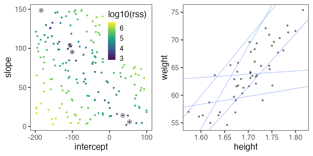
Can see a strong pattern: the taller the heavier
The relationship looks linear, $y = a x + b$.
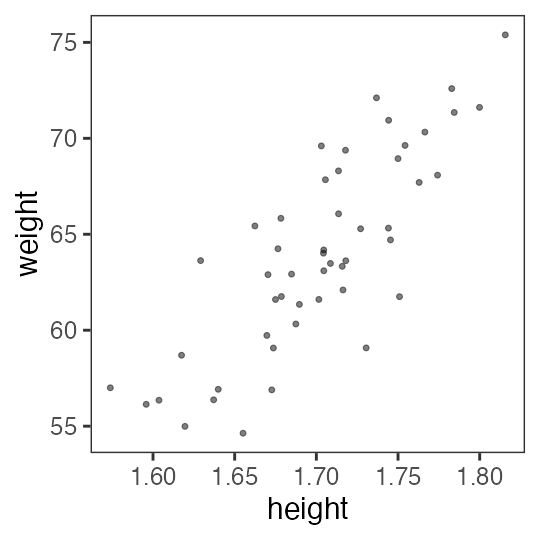
Can see a strong pattern: the taller the heavier
The relationship looks linear, $y = a x + b$.
OK, let’s try random slope a and intersect b:
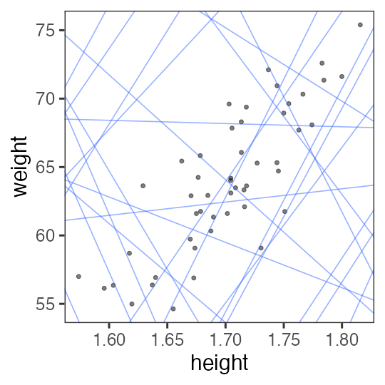
Need to find a good slope and intersect.
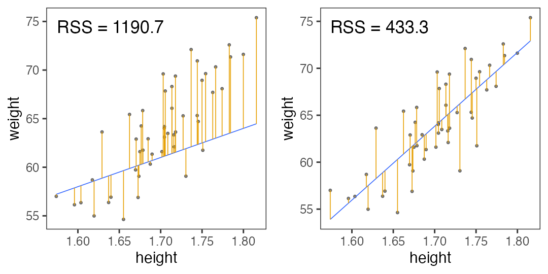
Ordinary Least Square (OLS)
minimizes the residual sum of squares (RSS) from the regression line.
Searching for models to minimize RSS
Try random values, and pick the best ones.
May need to generate much more to find good one.
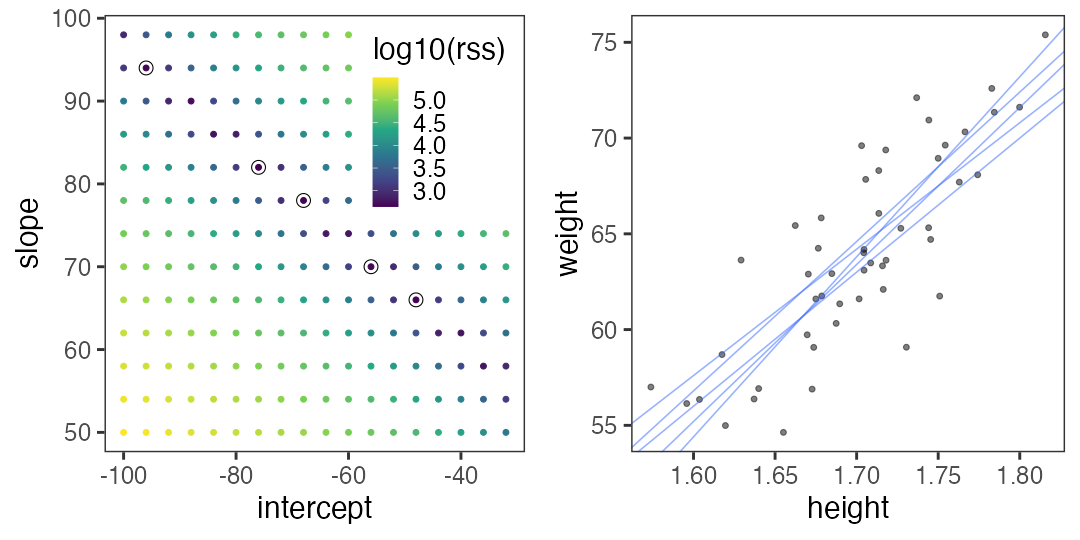
Searching for models to minimize RSS
Grid search: generate an evenly spaced grid of points.
Slightly more efficient than random search?
There are many other optimization techniques although not covered here.
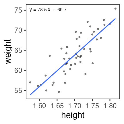
R can find the optimum in an instant
par_init = c(intercept = 0, slope = 0)
result = optim(par_init, fn = rss_weight, data = df_weight)
result$par
intercept     slope
-69.68394  78.53490
The code above is for general optimization.
For simple linear regression, an easier way is as follows…
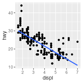
lm() function to fit linear models
fit = lm(data = mpg, formula = hwy ~ displ)
broom::tidy(fit)
         term  estimate std.error statistic       p.value
1 (Intercept) 35.697651 0.7203676  49.55477 2.123519e-125
2       displ -3.530589 0.1945137 -18.15085  2.038974e-46
mpg_added = modelr::add_predictions(mpg, fit, type = "response")
ggplot(mpg_added) + aes(displ, hwy) + geom_point() +
  geom_line(aes(y = pred), linewidth = 1, color = "#3366ff")
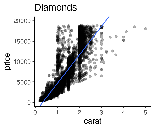
🔰 Try lm() with diamonds and iris.
Straight LM does not fit all
- Prediction goes below zero whereas all the observations are positive.
- Y values are integer. Their dispersion is larger when X is larger.
Straight LM does not fit all
- Prediction goes below zero whereas all the observations are positive.
- Y values are integer. Their dispersion is larger when X is larger.
- Let’s learn statistical modelling for better fitting to the data.
Extending linear regression
Linear Model (LM) 👈 #7 today
↓ probability distribution
Generalized Linear Model (GLM) — #8 next time
↓ individual difference, random effect
Generalized Linear Mixed Model (GLMM)
↓ flexible modelling
Hierarchical Bayesian Model (HBM)
「データ解析のための統計モデリング入門」久保拓弥 2012 より改変
Probability distribution
The relationship between phenomena and their frequencies.
- empirical distribution
- created by collecting samples.
- e.g., rolling a dice 12 times, heights of 1000 students:
- theoretical distribution
- described with math equation and a few parameters.
Random variable $X$ follows probability distribution $f$
$X \sim f(\theta)$
e.g.,
The number of heads in tossing 3 fair coins $X$ follows binomial distribution.
$X \sim \text{Binomial}(n = 3, p = 0.5)$
Let’s experiment.
Record repeated trials
The number of heads observed in tossing 3 fair coins: $X$
trial 1: H T H → $X = 2$
trial 2: T T T → $X = 0$
trial 3: H T T → $X = 1$, subsequently, $2, 1, 3, 0, 2, \ldots$
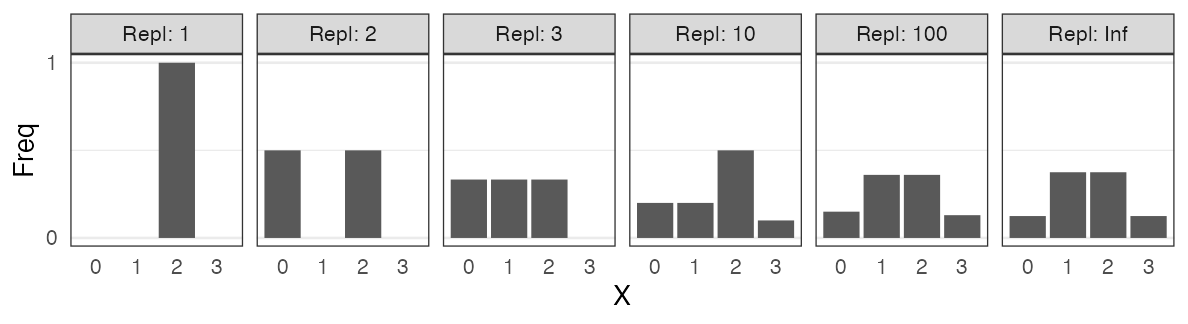
0 and 3 are rare. 1 and 2 are three times more likely.
Similar values can be generated without tossing coins
- The number of heads $X$ observed in tossing 3 fair coins.
- Random samples $X$ from the binomial distribution with $n = 3, p = 0.5$.

↓ sample
{2, 0, 1, 2, 1, 3, 0, 2, …}
These are so similar that we can say
“The number of heads in n tosses follows binomial distribution.”
Conversely, we can understand it like
“Random variable of binomial distribution is the number of successes in n trials.”
A kind of statistical modelling
Tossing 3 fair coins repeatedly {2, 0, 1, 2, 1, 3, 0, 2, …}
↑ simulate phenomena with a few parameters
Sample from binomial distribution with $n = 3, p = 0.5$

Any other probability distributions related to real phenomena like this?
Major probability distributions and related phenomena
- Discrete uniform distribution
- tossing fair coins, rolling fair dice
- Negative binomial distribution
(Geometric distribution if n = 1) - failures before the n-th success in trials with p
- Binomial distribution
- successes in n trials with p
- Poisson distribution
- occurrences of a Poisson process with $\lambda$
- Gamma distribution (Exponential distribution if k = 1)
- waiting time until k-th occurrence of a Poisson process with $\lambda$
- Normal/Gaussian distribution
- sum of random variables, sample means, etc.
Discrete uniform distribution
Every X in n values has equal probability $1/n$.
e.g., fair coin [0,1], fair dice [1,6]

🔰 Other examples of discrete uniform distribution?
Geometric distribution $~\text{Geom}(p)$
$X$ failures before the first success with success probability $p$ for each trial.
e.g., How many tails before first head with a coin?
\[ \Pr(X = k \mid p) = p (1 - p)^k \]
There is another definition: $X$ trials until the first success.
🔰 Other examples?
Negative binomial distribution $~\text{NB}(n, p)$
$X$ failures before the n-th success with success probability $p$ for each trial.
(identical to geometric distribution when n = 1)
\[ \Pr(X = k \mid n,~p) = \binom {n + k - 1} k p^n (1 - p)^k \]
There is another definition: $X$ trials until the n-th success.
🔰 Other examples?
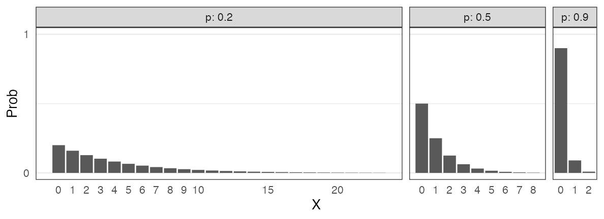
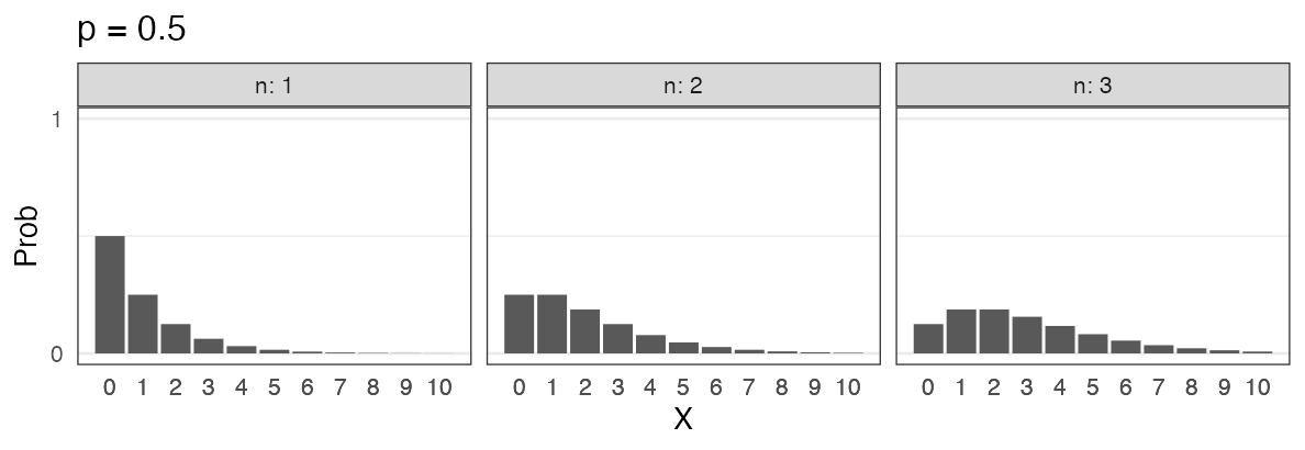
Binomial distribution $~\text{Binomial}(n,~p)$
$X$ successes in $n$ trials with success probability $p$ for each trial.
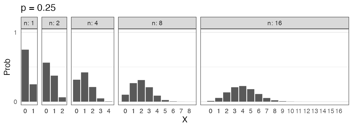
\[ \Pr(X = k \mid n,~p) = \binom n k p^k (1 - p)^{n - k} \]
🔰 Other examples?
Poisson distribution $~\text{Poisson}(\lambda)$
$X$ occurrences of a Poisson process in a fixed interval of time (space).
Poisson process: Events occur at a constant rate $\lambda$
e.g., messages received per hour, number of individuals in a quadrat
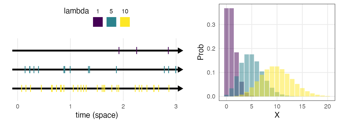
\[ \Pr(X = k \mid \lambda) = \frac {\lambda^k e^{-\lambda}} {k!} \]
The limit of binomial distribution $(\lambda = np;~n \to \infty;~p \to 0)$
≈ many trials of extremely rare events.
Exponential distribution $~\text{Exp}(\lambda)$
Interval $X$ between occurrences of a Poisson process.
Poisson process: Events occur at a constant rate $\lambda$
e.g., intervals between messages received, between gloves left on a road
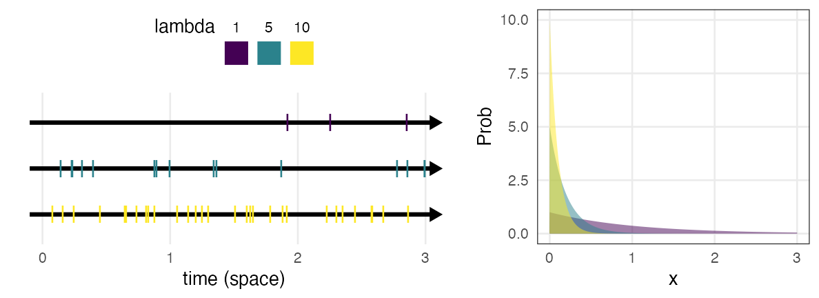
\[ \Pr(x \mid \lambda) = \lambda e^{-\lambda x} \]
The continuous counterpart of geometric distribution.
🔰 Other examples?
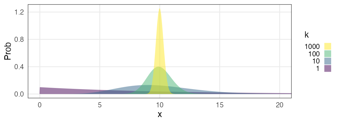
Gamma distribution $~\text{Gamma}(k,~\lambda)$
Waiting time $X$ until $k$-th occurrence of a Poisson process. Poisson process: Events occur at a constant rate $\lambda$
e.g., Waiting time until receiving two messages
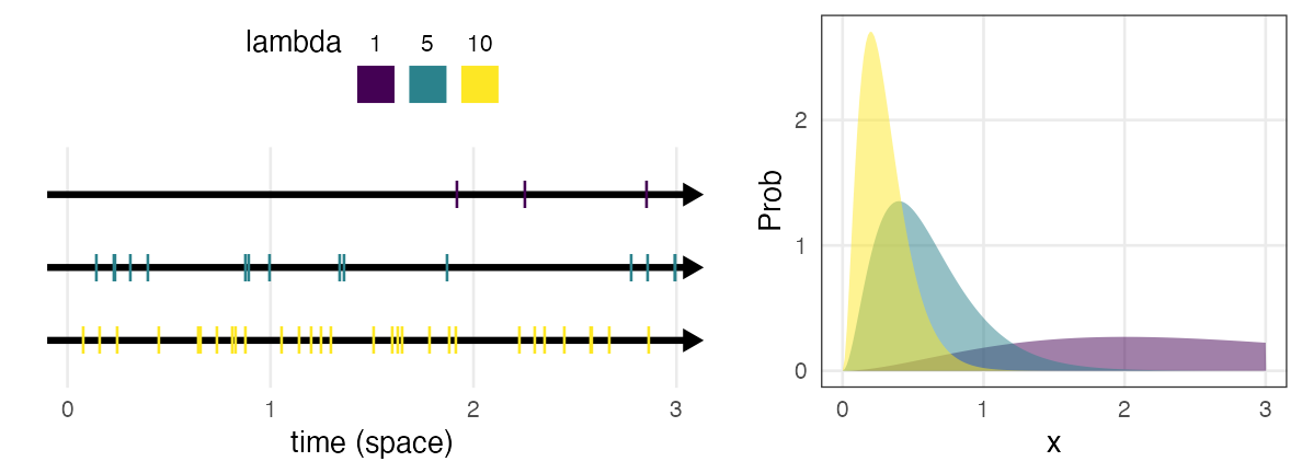
\[ \Pr(x \mid k,~\lambda) = \frac {\lambda^k x^{k - 1} e^{-\lambda x}} {\Gamma(k)} \]
Identical when shape parameter $k = 1$.
Normal/Gaussian distribution $~\mathcal{N}(\mu,~\sigma)$
Beautiful distribution with two parameters: mean $\mu$, standard deviation $\sigma$.
e.g., $\mu = 50, ~\sigma = 10$:
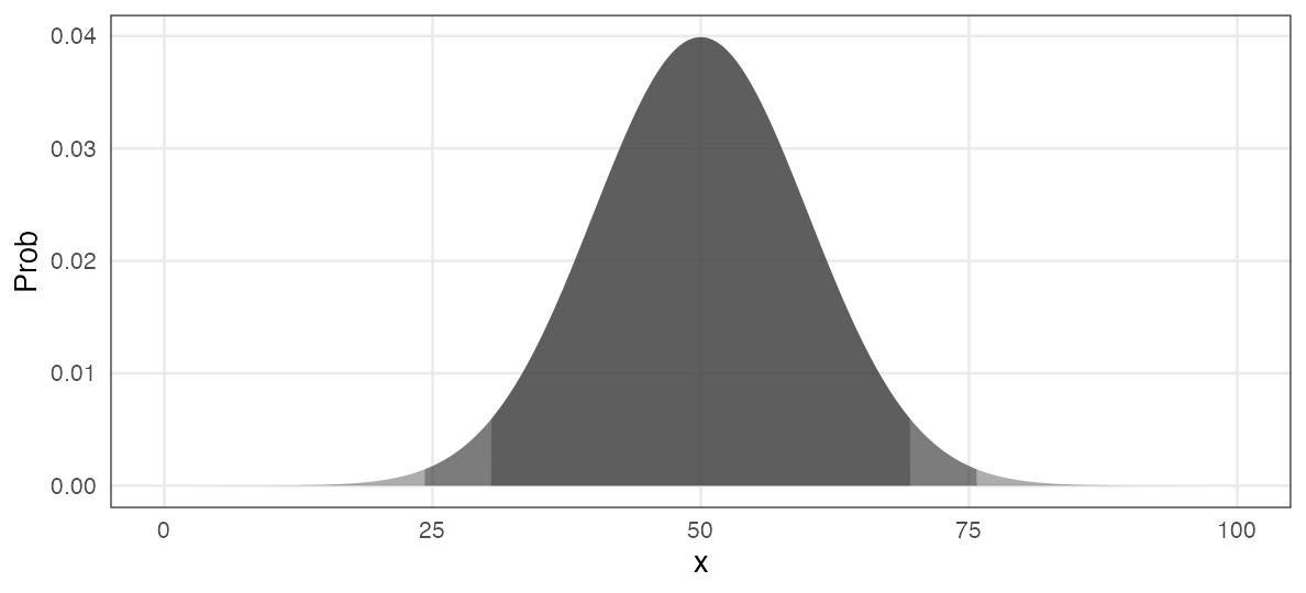
\[ \Pr(x \mid \mu,~\sigma) = \frac 1 {\sqrt{2 \pi \sigma^2}} \exp \left(\frac {-(x - \mu)^2} {2\sigma^2} \right) \]
Many distributions approach normal distribution
Distribution of sample means (central limit theorem); e.g., average of 40 samples from uniform distribution [0, 100):
Binomial distribution with large $n$:
Many distributions approach normal distribution
Poisson distribution with large $\lambda$:

Gamma distribution with large $k$:
Major probability distributions and related phenomena
- Discrete uniform distribution
- tossing fair coins, rolling fair dice
- Negative binomial distribution
(Geometric distribution if n = 1) - failures before the n-th success in trials with p
- Binomial distribution
- successes in n trials with p
- Poisson distribution
- occurrences of a Poisson process with $\lambda$
- Gamma distribution (Exponential distribution if k = 1)
- waiting time until k-th occurrence of a Poisson process with $\lambda$
- Normal/Gaussian distribution
- sum of random variables, sample means, etc.
Real data rarely follow theoretical distributions
Collect and sow 8 seeds from each of 100 plant individuals.
The number of survived seeds per parent should follow $\text{Binomial}(n = 8, p)$.
But extreme cases (all survived, all dead) were frequently observed.
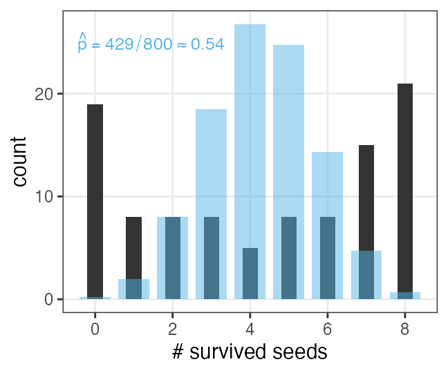
“Why? What other factors affect?” is the question of statistical modelling.
It requires the understanding of the null distribution.
Pseudo Random Number Generator
Algorithm to generate a sequence of random**-ish** numbers.
Its computation is not stochastic, but deterministic.
Exactly same values are generated if the same seed is set.
set.seed(42)
runif(3L)
# 0.9148060 0.9370754 0.2861395
runif(3L)
# 0.8304476 0.6417455 0.5190959
set.seed(42)
runif(6L)
# 0.9148060 0.9370754 0.2861395 0.8304476 0.6417455 0.5190959
Reproducible results can be obtained by fixing a seed.
Do NOT search for the seeds that produce favorable results.
Possible to generate various random numbers that follows probability distributions.
Generate random numbers from various distributions
n = 100
x = sample.int(6, n, replace = TRUE)
x = runif(n, min = 0, max = 1)
x = rgeom(n, prob = 0.5)
x = rbinom(n, size = 3, prob = 0.5)
x = rpois(n, lambda = 10)
x = rnorm(n, mean = 50, sd = 10)
print(x)

p1 = ggplot(data.frame(x)) + aes(x)
p1 + geom_histogram() # for continuous values
p1 + geom_bar()       # for discrete values
🔰 Observe the effects of altering sample size n.
🔰 Observe the effects of altering parameters for each distribution.
(Use Quarto effectively)
Fitting probability distributions to data
The number of seeds were counted for each of 50 plant individuals.
Individual A has 2 seeds, B has 4 seeds, …
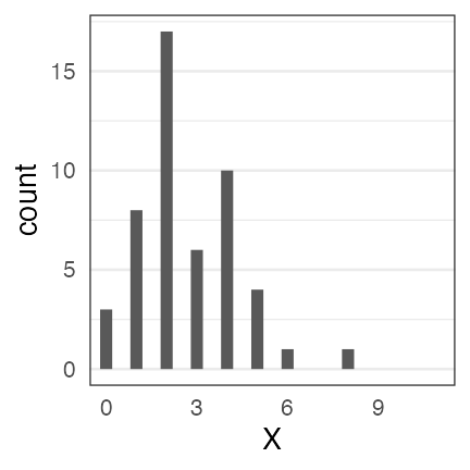
This count data looks Poisson-distributed.
What is the optimal $\lambda$ value?
Fitting probability distributions to data
The number of seeds were counted for each of 50 plant individuals.
Individual A has 2 seeds, B has 4 seeds, …
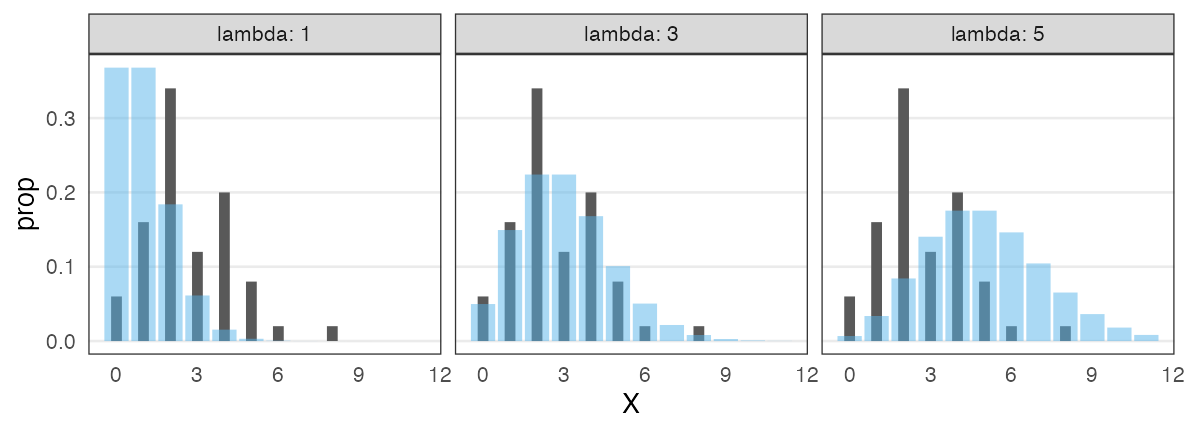
This count data looks Poisson-distributed.
What is the optimal $\lambda$ value?
Observations in black. Poisson distribution in blue. $\lambda = 3$ looks good.
Likelihood: a measure for goodness-of-fit
The probability to observe the data $D$ given the model $M$.
$\Pr(D \mid M)$
Likelihood function is the same probability from different viewpoints:
- as a function of model $M$ given the data $D$,
$L(M \mid D)$ - as a function of parameters $\theta$,
$L(\theta \mid D)$ or $L(\theta)$
Example of likelihood calculation
Data $D$: 4 heads (H) and 1 tail (T) in tossing a coin 5 times
Assuming the probability of coming up head $p = 0.5$:
Assuming the probability of coming up head $p = 0.8$:
$L(0.8 \mid D) > L(0.5 \mid D)$
$p = 0.8$ is more likely.
Likelihood in the example of Poisson distribution
The number of seeds were counted for each of 50 plant individuals.
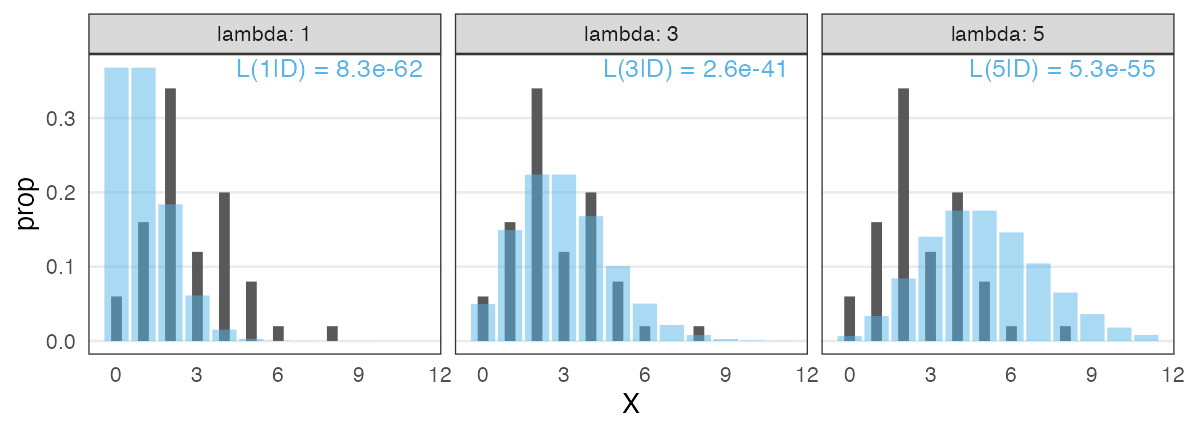
OK, $\lambda = 3$ is better than the other two. What is the best.
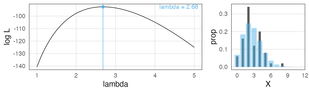
Maximum Likelihood Estimation
Log likelihood is often easier to handle.
Solving the differential equation for $\lambda$ …… finds the sample mean
MLE does not give you “true λ”
The data was actually generated from “$X \sim \text{Poisson}(\lambda = 3.0)$”.
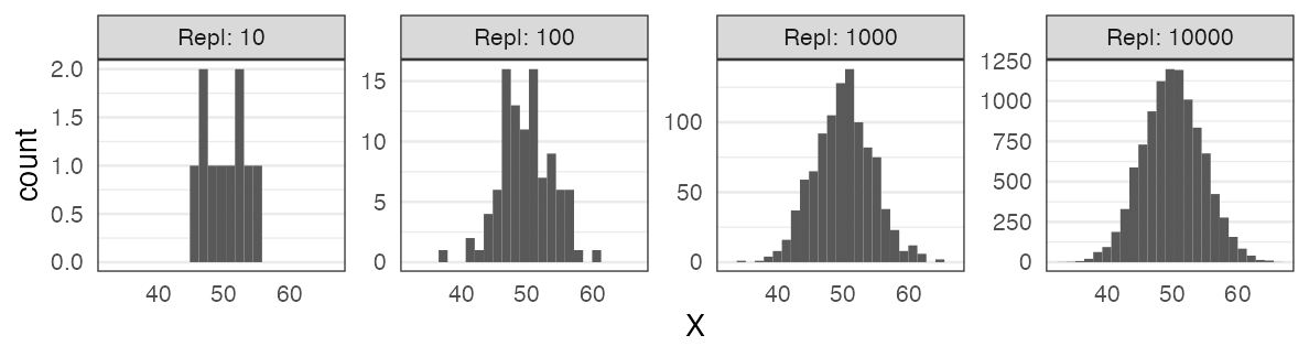
By replicating “sample 50 individuals → MLE” 1,000 times,
we find great variability in estimation and empirical distributions:
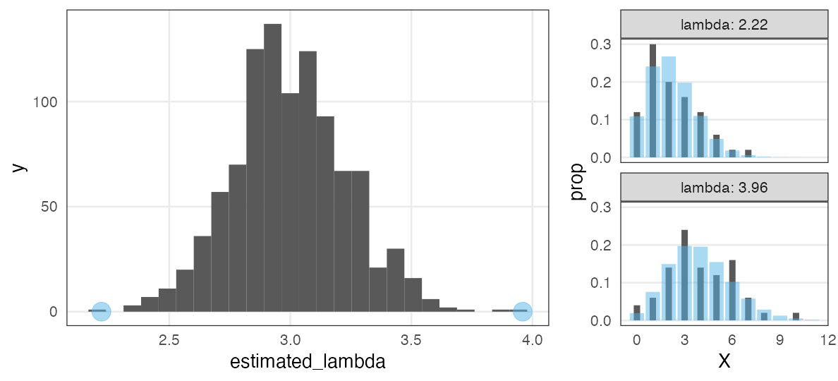
Note: Fitting to each sample looks not bad!
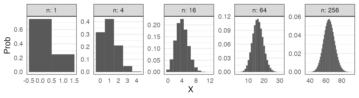
Alleviated by increasing sample size
1,000 replications of MLE with $n$ individuals from $X \sim \text{Poisson}(\lambda = 3.0)$:
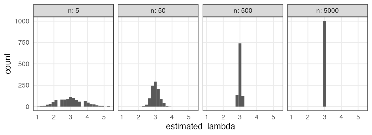
Q. How much is enough?
A. Depends on what you estimate, acceptable error range, etc.
Mathematical models in data science
All models are wrong, but some are useful. — George E. P. Box
Toolbox of statistical modelling
- Random variable $X$
- Probability distribution $X \sim f(\theta)$
- parameters $\theta$
- Likelihood
- The probability to observe the data given the model: $\Pr(D \mid M)$
- as a function of model given the data
→ likelihood function $L(M \mid D),~L(\theta \mid D)$ - Maximum Likelihood Estimation to fit parameters $\hat \theta$
🔰 Challenge: likelihood and MLE by hand
Rolling a dice 10 times, 3 sixes were observed.
-
Calculate likelihood assuming the probability to come up 6 $p = 1/6$.
-
Calculate likelihood assuming the probability to come up 6 $p = 0.2$.
-
Draw a graph with $p$ as horizontal axis, log likelihood as vertical axis.
-
Estimate $p$ with MLE.
Excellent, if solved with math; Good, if solved with R; OK, by eye or intuition.
- Hint
- $\binom 5 2 = {}_5 \mathrm{C} _2 = 10$ can be achieved with
choose(5, 2)in R.
Reference
- データ解析のための統計モデリング入門 久保拓弥 2012
- StanとRでベイズ統計モデリング 松浦健太郎 2016
- RとStanではじめる ベイズ統計モデリングによるデータ分析入門 馬場真哉 2019
- データ分析のための数理モデル入門 江崎貴裕 2020
- 分析者のためのデータ解釈学入門 江崎貴裕 2020
- 統計学を哲学する 大塚淳 2020
- 科学とモデル—シミュレーションの哲学 入門 Michael Weisberg 2017
(原著: Simulation and Similarity 2013)