Hands-on Introduction to R 2023
- Introduction: what is data analysis and R basics
- Data visualization and reporting
- Data transformation 1: extract, summarize
- Data transformation 2: join, pivot
- Data cleansing and conversion: numbers, text
- Data input and interpretation
- Statistical modeling 1: probability distribution, likelihood
- Statistical modeling 2: linear regression
https://heavywatal.github.io/slides/english2023r/
Purposes of this hands-on lectures
✅ Every biological research involves data and models
✅ You want to do reproducible analysis
⬜ Learn how to do it and how to learn more
- Overview what R can do.
- Know where to consult when you have a problem.
⬜ Glance at the basics of data analysis
You don’t have to remember every command.
Just repeat forgetting and searching.
Outline of data analysis
- Setup computer environment ✅
- Get and read input data ⬜ day 6
- Exploratory data analysis
- Preparation (harder than it seems) ⬜ day 3–5 👈
- Visualization, generating hypotheses (fun!) ✅ day 2
- Statistical analysis, testing hypotheses ⬜ day 7–8
- Report ✅ day 2
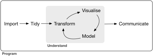
Now we know visualization is very important
reorganization of information → proper analysis, new hypotheses
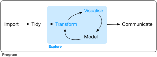
But it is rare that you get data in the right form to draw graphs.
Some say,
data scientists spend 80% of their resources for data preparation.
Machine process ≠ Human read/write
- Similar data formats required for visualization and analysis
ggplot(data, ...),glm(..., data, ...), …- Different data formats from source to source
- lab notebooks, fieldnotes, databases, etc.
Happy families are all alike;
every unhappy family is unhappy in its own way
tidy datasets are all alike,
but every messy dataset is messy in its own way
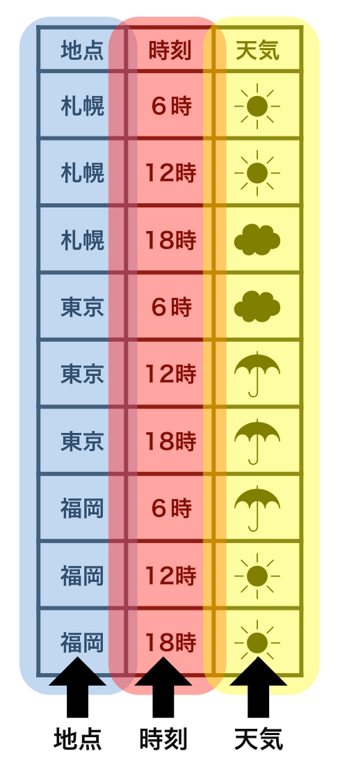
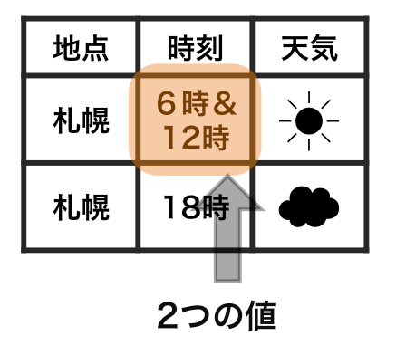
tidy data vs messy data
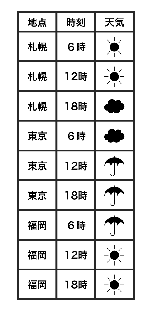
Each row is an observation.
Each cell is a single value.
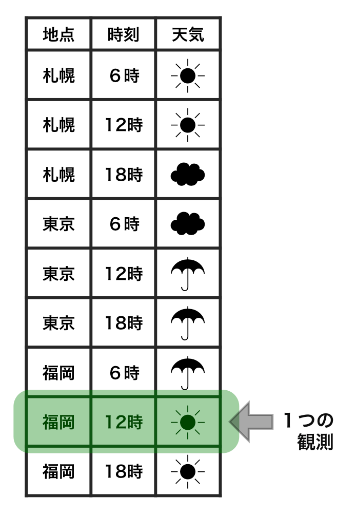
tidy data vs messy data
Each row is an observation.
Each cell is a single value.
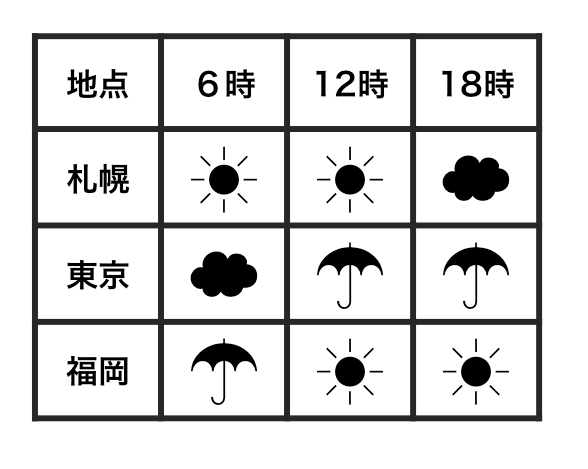
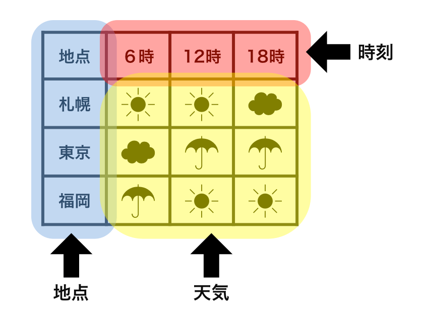
tidy data vs messy data
Each row is an observation.
Each cell is a single value.
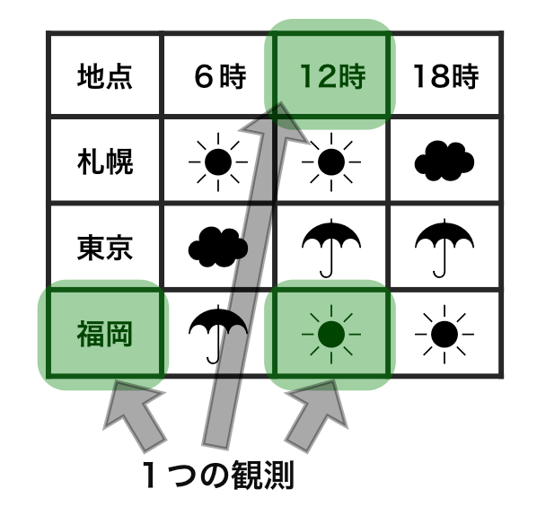
tidy data vs messy data
Each row is an observation.
Each cell is a single value.
tidy data ≈ data.frame tempting you to ggplot
- Each column is a variable.
- Each row is an observation.
- Each cell is a single value.
https://r4ds.hadley.nz/data-tidy.html
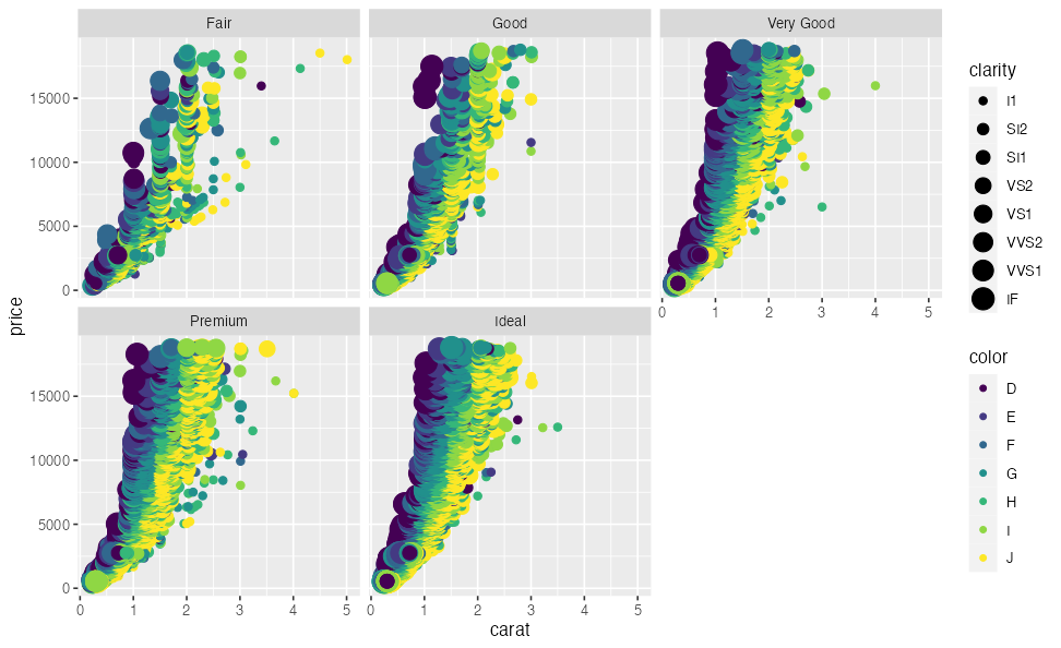
print(ggplot2::diamonds)
      carat       cut color clarity depth table price    x    y    z
    1  0.23     Ideal     E     SI2  61.5    55   326 3.95 3.98 2.43
    2  0.21   Premium     E     SI1  59.8    61   326 3.89 3.84 2.31
    3  0.23      Good     E     VS1  56.9    65   327 4.05 4.07 2.31
    4  0.29   Premium     I     VS2  62.4    58   334 4.20 4.23 2.63
   --
53937  0.72      Good     D     SI1  63.1    55  2757 5.69 5.75 3.61
53938  0.70 Very Good     D     SI1  62.8    60  2757 5.66 5.68 3.56
53939  0.86   Premium     H     SI2  61.0    58  2757 6.15 6.12 3.74
53940  0.75     Ideal     D     SI2  62.2    55  2757 5.83 5.87 3.64
tidy data ≈ data.frame tempting you to ggplot
Aesthetic mapping and faceting by column names:
ggplot(diamonds) + aes(x = carat, y = price) +
  geom_point(mapping = aes(color = color, size = clarity)) +
  facet_wrap(vars(cut))
Immediate goal: skills to prepare tidy data
print(VADeaths)
      Rural Male Rural Female Urban Male Urban Female
50-54       11.7          8.7       15.4          8.4
55-59       18.1         11.7       24.3         13.6
60-64       26.9         20.3       37.0         19.3
65-69       41.0         30.9       54.6         35.1
70-74       66.0         54.3       71.1         50.0
↓ mise en place 🔪 put everything in place
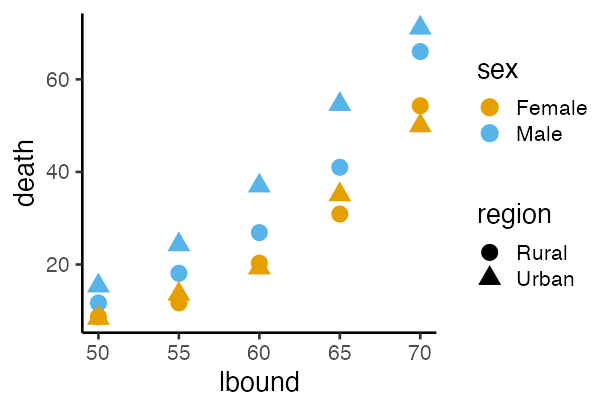
   lbound ubound region    sex death
 1     50     54  Rural   Male  11.7
 2     50     54  Rural Female   8.7
 3     50     54  Urban   Male  15.4
 4     50     54  Urban Female   8.4
--
17     70     74  Rural   Male  66.0
18     70     74  Rural Female  54.3
19     70     74  Urban   Male  71.1
20     70     74  Urban Female  50.0
Learning data preparation in two categories
- Processing data structure 👈 day 3 and 4
- Extract subsets
- Summarize by group
- Sort rows
- Combine tables
- Pivot longer ↔ wider
- Processing data content — day 5
- Type conversion: continuous vs discrete, factors, time
- Mathematical conversion: logarithm, normalization
- Handling outliers and missing values
- Character manipulation: pattern matching
tidyverse: a collection of R packages for data science
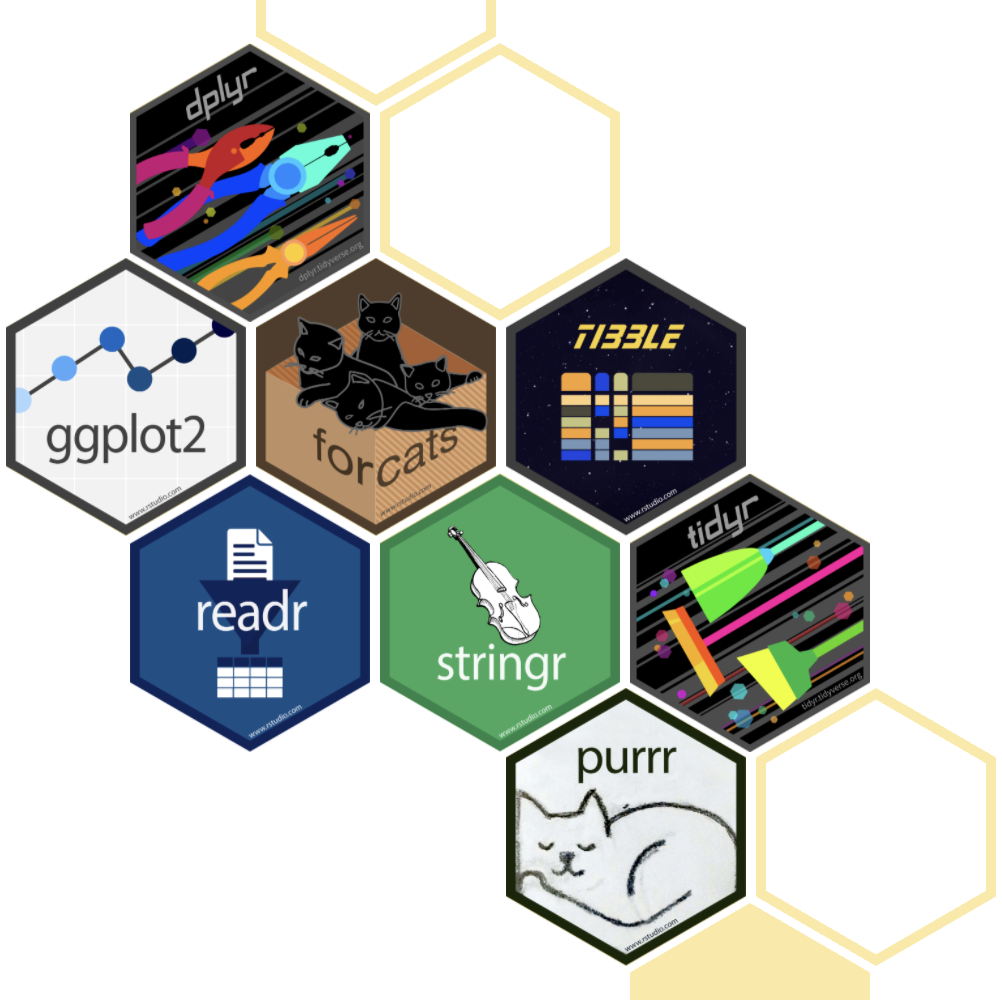
install.packages("tidyverse")
library(conflicted) # charm for safe coding
library(tidyverse)  # load core packages at once
── Attaching core tidyverse packages ──── tidyverse 2.0.0 ──
✔ dplyr     1.1.4     ✔ readr     2.1.5
✔ forcats   1.0.0     ✔ stringr   1.5.1
✔ ggplot2   3.5.1     ✔ tibble    3.2.1
✔ lubridate 1.9.4     ✔ tidyr     1.3.1
✔ purrr     1.0.4
Consistently designed to cover all the processes in data analysis.
dplyr — plyer for data.frames

A consistent set of verbs/functions for data manipulation.
- Extract
- columns:
select(), - rows:
filter(),distinct(),slice() - Aggregate
group_by(),summarize(),count()- Reorder
arrange(),relocate()- Modify/add columns
mutate(),rename()- Join/bind
- rows:
bind_rows() - columns:
left_join(),inner_join(),full_join()
Getting ready to use dplyr
Load packages. Take a look at the data:
# install.packages("tidyverse")
library(conflicted) # charm for safe coding
library(tidyverse)  # load packages including ggplot2, dplyr
print(diamonds)
View(diamonds)  # RStudio
      carat       cut color clarity depth table price    x    y    z
    1  0.23     Ideal     E     SI2  61.5    55   326 3.95 3.98 2.43
    2  0.21   Premium     E     SI1  59.8    61   326 3.89 3.84 2.31
    3  0.23      Good     E     VS1  56.9    65   327 4.05 4.07 2.31
    4  0.29   Premium     I     VS2  62.4    58   334 4.20 4.23 2.63
   --
53937  0.72      Good     D     SI1  63.1    55  2757 5.69 5.75 3.61
53938  0.70 Very Good     D     SI1  62.8    60  2757 5.66 5.68 3.56
53939  0.86   Premium     H     SI2  61.0    58  2757 6.15 6.12 3.74
53940  0.75     Ideal     D     SI2  62.2    55  2757 5.83 5.87 3.64
🔰 View also starwars data.
Use explicit namespace dplyr::
There are conflicts between same-named functions from different packages.
library(conflicted) makes every conflict an error for safety:
filter(diamonds, carat > 4.2)
Error: ! [conflicted] filter found in 2 packages.
Either pick the one you want with `::`:
• dplyr::filter
• stats::filter
Or declare a preference with `conflicts_prefer()`:
• `conflicts_prefer(dplyr::filter)`
• `conflicts_prefer(stats::filter)`
Follow the instruction, and use :: operator:
dplyr::filter(diamonds, carat > 4.2)
  carat  cut color clarity depth table price     x     y    z
1  5.01 Fair     J      I1  65.5    59 18018 10.74 10.54 6.98
2  4.50 Fair     J      I1  65.8    58 18531 10.23 10.16 6.72
Typical usage of dplyr functions
Apply small functions like assembly-line operations:
result = diamonds |>                   # start
  dplyr::select(carat, cut, price) |>  # extract columns
  dplyr::filter(carat > 1) |>          # extract rows
  dplyr::group_by(cut) |>              # split internally
  dplyr::summarize(mean(price)) |>     # average by group
  print()                              # output to console
        cut mean(price)
1      Fair    7177.856
2      Good    7753.601
3 Very Good    8340.549
4   Premium    8487.249
5     Ideal    8674.227
What is this unfamiliar |> operator?
(Each function will be explained later.)
Pipe operator |>
puts the variable on the left into the first argument of the function on the right:
# These two lines are equivalent
diamonds |> filter(carat > 1)
filter(diamonds, carat > 1)

# useful for assembly-line:
diamonds |> filter(carat > 1) |> select(carat, price) |> ...
potatoes |> cut() |> fry() |> season("salt") |> eat()
🔰 Translate the following code not to use the pipe:
seq(1, 6) |> sum()
[1] 21
letters |> toupper() |> head(3)
[1] "A" "B" "C"
[example solution]
sum(seq(1, 6))
head(toupper(letters), 3)
If we didn’t have the pipe |>
😐 Create temporary objects every time:
tmp1 = dplyr::select(diamonds, carat, cut, price) # extract columns
tmp2 = dplyr::filter(tmp1, carat > 1)             # extract rows
tmp3 = dplyr::group_by(tmp2, cut)                 # split internally
result = dplyr::summarize(tmp3, mean(price))      # average by group
😐 Reuse the same name again and again:
result = dplyr::select(diamonds, carat, cut, price) # extract columns
result = dplyr::filter(result, carat > 1)           # extract rows
result = dplyr::group_by(result, cut)               # split internally
result = dplyr::summarize(result, mean(price))      # average by group
Not too bad. But a bit redundant to repeat variable names many times.
If we didn’t have the pipe |>
😫 Get over without temporary objects:
result = dplyr::summarize(              # average by group
    dplyr::group_by(                        # split internally
      dplyr::filter(                            # extract rows
        dplyr::select(diamonds, carat, cut, price), # extract columns
        carat > 1),                             # extract rows
      cut),                                 # split internally
    mean(price))                        # average by group
🤪 even without line breaks:
result = dplyr::summarize(dplyr::group_by(dplyr::filter(dplyr::select(diamonds, carat, cut, price), carat > 1), cut), mean(price))
They require erratic eye movements.
Worse than the previous ones.
Let’s use the pipe |>
😁 Much easier to follow the logical flow from top to bottom:
result = diamonds |>                   # start
  dplyr::select(carat, cut, price) |>  # extract columns
  dplyr::filter(carat > 1) |>          # extract rows
  dplyr::group_by(cut) |>              # split internally
  dplyr::summarize(mean(price)) |>     # average by group
  print()                              # output to console
        cut mean(price)
1      Fair    7177.856
2      Good    7753.601
3 Very Good    8340.549
4   Premium    8487.249
5     Ideal    8674.227
It may take an extra effort to get used to it, but it’s worth it.
tidyverse packages are designed to be used with the pipe.
%>% is almost the same. It was widely used when R < 4.2.
select() columns
based on their numbers:
result = diamonds |>
  dplyr::select(1, 2, 7) |>
  print()
      carat       cut price
    1  0.23     Ideal   326
    2  0.21   Premium   326
    3  0.23      Good   327
    4  0.29   Premium   334
   --
53937  0.72      Good  2757
53938  0.70 Very Good  2757
53939  0.86   Premium  2757
53940  0.75     Ideal  2757
other solutions: |> dplyr::select(c(1, 2, 7)), diamonds[, c(1, 2, 7)]
🔰 Extract the columns 1, 10, 11 from starwars in three ways.
select() columns
based on their names:
result = diamonds |>
  dplyr::select(carat, cut, price) |>
  print()
      carat       cut price
    1  0.23     Ideal   326
    2  0.21   Premium   326
    3  0.23      Good   327
    4  0.29   Premium   334
   --
53937  0.72      Good  2757
53938  0.70 Very Good  2757
53939  0.86   Premium  2757
53940  0.75     Ideal  2757
another solution: |> dplyr::select(c("carat", "cut", "price"))
🔰 Extract the columns 1, 10, 11 from starwars based on their names.
select() columns
to discard:
result = diamonds |>
  dplyr::select(!c(carat, cut, price)) |>
  print()
      color clarity depth table    x    y    z
    1     E     SI2  61.5    55 3.95 3.98 2.43
    2     E     SI1  59.8    61 3.89 3.84 2.31
    3     E     VS1  56.9    65 4.05 4.07 2.31
    4     I     VS2  62.4    58 4.20 4.23 2.63
   --
53937     D     SI1  63.1    55 5.69 5.75 3.61
53938     D     SI1  62.8    60 5.66 5.68 3.56
53939     H     SI2  61.0    58 6.15 6.12 3.74
53940     D     SI2  62.2    55 5.83 5.87 3.64
another solution: |> dplyr::select(!c("carat", "cut", "price"))
🔰 Exclude the columns 1, 10, 11 from starwars.
select() columns
based on the partial match of their names:
result = diamonds |>
  dplyr::select(starts_with("c")) |>
  print()
      carat       cut color clarity
    1  0.23     Ideal     E     SI2
    2  0.21   Premium     E     SI1
    3  0.23      Good     E     VS1
    4  0.29   Premium     I     VS2
   --
53937  0.72      Good     D     SI1
53938  0.70 Very Good     D     SI1
53939  0.86   Premium     H     SI2
53940  0.75     Ideal     D     SI2
See ?dplyr_tidy_select or selection helpers for more details.
🔰 Extract the columns whose name ends with “s” from starwars
select() columns
based on data types:
result = diamonds |>
  dplyr::select(where(is.numeric)) |>
  print()
      carat depth table price    x    y    z
    1  0.23  61.5    55   326 3.95 3.98 2.43
    2  0.21  59.8    61   326 3.89 3.84 2.31
    3  0.23  56.9    65   327 4.05 4.07 2.31
    4  0.29  62.4    58   334 4.20 4.23 2.63
   --
53937  0.72  63.1    55  2757 5.69 5.75 3.61
53938  0.70  62.8    60  2757 5.66 5.68 3.56
53939  0.86  61.0    58  2757 6.15 6.12 3.74
53940  0.75  62.2    55  2757 5.83 5.87 3.64
See ?dplyr_tidy_select or tidyselect::where for more details.
🔰 Extract character columns from starwars.
filter() rows
based on the exact match (==) of their values:
result = diamonds |>
  dplyr::filter(cut == "Ideal") |>
  print()
      carat   cut color clarity depth table price    x    y    z
    1  0.23 Ideal     E     SI2  61.5    55   326 3.95 3.98 2.43
    2  0.23 Ideal     J     VS1  62.8    56   340 3.93 3.90 2.46
    3  0.31 Ideal     J     SI2  62.2    54   344 4.35 4.37 2.71
    4  0.30 Ideal     I     SI2  62.0    54   348 4.31 4.34 2.68
   --
21548  0.71 Ideal     E     SI1  61.9    56  2756 5.71 5.73 3.54
21549  0.71 Ideal     G     VS1  61.4    56  2756 5.76 5.73 3.53
21550  0.72 Ideal     D     SI1  60.8    57  2757 5.75 5.76 3.50
21551  0.75 Ideal     D     SI2  62.2    55  2757 5.83 5.87 3.64
another solution: diamonds[diamonds[["cut"]] == "Ideal", ]
🔰 Extract humans from starwars.
filter() rows
that satisfy the inequality (!=, <, <=, >, >=):
result = diamonds |>
  dplyr::filter(cut != "Ideal") |>
  print()
      carat       cut color clarity depth table price    x    y    z
    1  0.21   Premium     E     SI1  59.8    61   326 3.89 3.84 2.31
    2  0.23      Good     E     VS1  56.9    65   327 4.05 4.07 2.31
    3  0.29   Premium     I     VS2  62.4    58   334 4.20 4.23 2.63
    4  0.31      Good     J     SI2  63.3    58   335 4.34 4.35 2.75
   --
32386  0.72   Premium     D     SI1  62.7    59  2757 5.69 5.73 3.58
32387  0.72      Good     D     SI1  63.1    55  2757 5.69 5.75 3.61
32388  0.70 Very Good     D     SI1  62.8    60  2757 5.66 5.68 3.56
32389  0.86   Premium     H     SI2  61.0    58  2757 6.15 6.12 3.74
🔰 Extract characters shorter than 150 from starwars.
filter() rows
with values that match any of the given values:
result = diamonds |>
  dplyr::filter(cut %in% c("Ideal", "Good")) |>
  print()
      carat   cut color clarity depth table price    x    y    z
    1  0.23 Ideal     E     SI2  61.5    55   326 3.95 3.98 2.43
    2  0.23  Good     E     VS1  56.9    65   327 4.05 4.07 2.31
    3  0.31  Good     J     SI2  63.3    58   335 4.34 4.35 2.75
    4  0.30  Good     J     SI1  64.0    55   339 4.25 4.28 2.73
   --
26454  0.71 Ideal     G     VS1  61.4    56  2756 5.76 5.73 3.53
26455  0.72 Ideal     D     SI1  60.8    57  2757 5.75 5.76 3.50
26456  0.72  Good     D     SI1  63.1    55  2757 5.69 5.75 3.61
26457  0.75 Ideal     D     SI2  62.2    55  2757 5.83 5.87 3.64
🔰 Extract characters whose eyes are blue or red from starwars.
filter() rows
that satisfy both of the given conditions (AND):
result = diamonds |>
  dplyr::filter(carat > 2 & price < 14000) |>
  print()
    carat       cut color clarity depth table price    x    y    z
  1  2.06   Premium     J      I1  61.2    58  5203 8.10 8.07 4.95
  2  2.14      Fair     J      I1  69.4    57  5405 7.74 7.70 5.36
  3  2.15      Fair     J      I1  65.5    57  5430 8.01 7.95 5.23
  4  2.22      Fair     J      I1  66.7    56  5607 8.04 8.02 5.36
 --
641  2.07   Premium     H     SI1  62.7    58 13993 8.14 8.09 5.09
642  2.07      Good     I     SI1  63.6    58 13993 8.09 7.99 5.11
643  2.13 Very Good     J     SI1  62.8    58 13996 8.13 8.17 5.12
644  2.11   Premium     J     SI1  62.4    58 13996 8.27 8.17 5.13
🔰 Extract humans whose homeworld is Tatooine from starwars.
filter() rows
that satisfy either of the given conditions (OR):
result = diamonds |>
  dplyr::filter(carat > 2 | price < 14000) |>
  print()
      carat       cut color clarity depth table price    x    y    z
    1  0.23     Ideal     E     SI2  61.5    55   326 3.95 3.98 2.43
    2  0.21   Premium     E     SI1  59.8    61   326 3.89 3.84 2.31
    3  0.23      Good     E     VS1  56.9    65   327 4.05 4.07 2.31
    4  0.29   Premium     I     VS2  62.4    58   334 4.20 4.23 2.63
   --
53023  0.72      Good     D     SI1  63.1    55  2757 5.69 5.75 3.61
53024  0.70 Very Good     D     SI1  62.8    60  2757 5.66 5.68 3.56
53025  0.86   Premium     H     SI2  61.0    58  2757 6.15 6.12 3.74
53026  0.75     Ideal     D     SI2  62.2    55  2757 5.83 5.87 3.64
🔰 Extract those taller than 200 or heavier than 100 from starwars.
slice_max(), slice_min()
extract rows with the largest values of the given columns:
result = diamonds |>
  dplyr::slice_max(price, n = 5L) |>
  print()
  carat       cut color clarity depth table price    x    y    z
1  2.29   Premium     I     VS2  60.8    60 18823 8.50 8.47 5.16
2  2.00 Very Good     G     SI1  63.5    56 18818 7.90 7.97 5.04
3  1.51     Ideal     G      IF  61.7    55 18806 7.37 7.41 4.56
4  2.07     Ideal     G     SI2  62.5    55 18804 8.20 8.13 5.11
5  2.00 Very Good     H     SI1  62.8    57 18803 7.95 8.00 5.01
Provide n or prop to set the number/proportion of rows.
🔰 Extract the shortest five characters from starwars.
slice_max(), slice_min()
extract rows with the largest values from each group:
result = diamonds |>
  dplyr::group_by(cut) |>
  dplyr::slice_max(price, n = 2L) |>
  print()
   carat     cut color clarity depth table price    x    y    z
 1  2.01    Fair     G     SI1  70.6    64 18574 7.43 6.64 4.69
 2  2.02    Fair     H     VS2  64.5    57 18565 8.00 7.95 5.14
 3  2.80    Good     G     SI2  63.8    58 18788 8.90 8.85 0.00
 4  2.07    Good     I     VS2  61.8    61 18707 8.12 8.16 5.03
--
 7  2.29 Premium     I     VS2  60.8    60 18823 8.50 8.47 5.16
 8  2.29 Premium     I     SI1  61.8    59 18797 8.52 8.45 5.24
 9  1.51   Ideal     G      IF  61.7    55 18806 7.37 7.41 4.56
10  2.07   Ideal     G     SI2  62.5    55 18804 8.20 8.13 5.11
🔰 Extract the shortest three rows for each gender from starwars.
slice_head(), slice_tail()
extract the first/last n rows from each group:
result = diamonds |>
  dplyr::group_by(cut) |>
  dplyr::slice_head(n = 3L) |>
  print()
   carat     cut color clarity depth table price    x    y    z
 1  0.22    Fair     E     VS2  65.1    61   337 3.87 3.78 2.49
 2  0.86    Fair     E     SI2  55.1    69  2757 6.45 6.33 3.52
 3  0.96    Fair     F     SI2  66.3    62  2759 6.27 5.95 4.07
 4  0.23    Good     E     VS1  56.9    65   327 4.05 4.07 2.31
--
12  0.22 Premium     F     SI1  60.4    61   342 3.88 3.84 2.33
13  0.23   Ideal     E     SI2  61.5    55   326 3.95 3.98 2.43
14  0.23   Ideal     J     VS1  62.8    56   340 3.93 3.90 2.46
15  0.31   Ideal     J     SI2  62.2    54   344 4.35 4.37 2.71
Provide n or prop to set the number/proportion of rows.
🔰 Extract the first three rows for each gender from starwars.
slice_sample()
extract n rows randomly from each group:
result = diamonds |>
  dplyr::group_by(cut) |>
  dplyr::slice_sample(n = 3L, replace = FALSE) |>
  print()
   carat     cut color clarity depth table price    x    y    z
 1  0.45    Fair     F     SI1  66.8    59   794 4.79 4.63 3.16
 2  0.90    Fair     E     SI2  65.8    58  3084 6.02 5.98 3.95
 3  2.00    Fair     J     VS2  65.4    58 11966 7.96 7.75 5.14
 4  2.18    Good     H     SI2  60.4    64 16690 8.38 8.47 5.09
--
12  0.80 Premium     G     SI2  61.4    56  2451 5.99 5.96 3.67
13  1.58   Ideal     E     VS2  62.7    56 15579 7.45 7.55 4.70
14  0.53   Ideal     F    VVS2  62.7    56  2030 5.16 6.20 3.25
15  1.10   Ideal     G    VVS2  60.5    56  9215 6.76 6.70 4.07
🔰 Extract the three rows for each gender randomly from starwars.
slice()
extract arbitrary rows from each group:
result = diamonds |>
  dplyr::group_by(cut) |>
  dplyr::slice(c(1, 2, 9)) |>
  print()
   carat     cut color clarity depth table price    x    y    z
 1  0.22    Fair     E     VS2  65.1    61   337 3.87 3.78 2.49
 2  0.86    Fair     E     SI2  55.1    69  2757 6.45 6.33 3.52
 3  0.84    Fair     G     SI1  55.1    67  2782 6.39 6.20 3.47
 4  0.23    Good     E     VS1  56.9    65   327 4.05 4.07 2.31
--
12  0.22 Premium     D     VS2  59.3    62   404 3.91 3.88 2.31
13  0.23   Ideal     E     SI2  61.5    55   326 3.95 3.98 2.43
14  0.23   Ideal     J     VS1  62.8    56   340 3.93 3.90 2.46
15  0.32   Ideal     I     SI1  60.9    55   404 4.45 4.48 2.72
summarize()
calculate the sum, mean, maximum of the given columns:
result = diamonds |>
  dplyr::summarize(sum(carat), mean(carat), max(price)) |>
  print()
  sum(carat) mean(carat) max(price)
1   43040.87   0.7979397      18823
aggregate functions that receive a vector and return a single value:
min(), max(), mean(), median(), var(), sd(), etc.
🔰 Calculate average cty and hwy of mpg.
summarize()
for each group:
result = diamonds |>
  dplyr::group_by(cut) |>
  dplyr::summarize(avg_carat = mean(carat),
                   max_price = max(price)) |>
  print()
        cut avg_carat max_price
1      Fair 1.0461366     18574
2      Good 0.8491847     18788
3 Very Good 0.8063814     18818
4   Premium 0.8919549     18823
5     Ideal 0.7028370     18806
🔰 Calculate average cty and hwy for each drv of mpg.
summarize(across())
multiple columns at once:
result = diamonds |>
  dplyr::group_by(cut) |>
  dplyr::summarize(across(where(is.numeric), mean)) |>
  print()
        cut     carat    depth    table    price        x        y        z
1      Fair 1.0461366 64.04168 59.05379 4358.758 6.246894 6.182652 3.982770
2      Good 0.8491847 62.36588 58.69464 3928.864 5.838785 5.850744 3.639507
3 Very Good 0.8063814 61.81828 57.95615 3981.760 5.740696 5.770026 3.559801
4   Premium 0.8919549 61.26467 58.74610 4584.258 5.973887 5.944879 3.647124
5     Ideal 0.7028370 61.70940 55.95167 3457.542 5.507451 5.520080 3.401448
🔰 Pick the maximum value for each numeric column in mpg.
reframe()
summarizes each group to an arbitrary number of rows:
quantile(diamonds$price)
      0%      25%      50%      75%     100%
  326.00   950.00  2401.00  5324.25 18823.00
result = diamonds |>
  dplyr::reframe(across(where(is.numeric), quantile)) |>
  print()
  carat depth table    price     x     y     z
1  0.20  43.0    43   326.00  0.00  0.00  0.00
2  0.40  61.0    56   950.00  4.71  4.72  2.91
3  0.70  61.8    57  2401.00  5.70  5.71  3.53
4  1.04  62.5    59  5324.25  6.54  6.54  4.04
5  5.01  79.0    95 18823.00 10.74 58.90 31.80
🔰 Apply range() to all the numeric columns for each drv in mpg.
count() occurrences
of the combination of given columns:
result = diamonds |>
  dplyr::count(cut, color) |>
  print()
     cut color    n
 1  Fair     D  163
 2  Fair     E  224
 3  Fair     F  312
 4  Fair     G  314
--
32 Ideal     G 4884
33 Ideal     H 3115
34 Ideal     I 2093
35 Ideal     J  896
🔰 Count the combinations of sex and gender in starwars.
Keep only distinct() rows
regarding the given columns:
result = diamonds |>
  dplyr::distinct(cut, color) |>
  print()
       cut color
 1   Ideal     E
 2 Premium     E
 3    Good     E
 4 Premium     I
--
32    Fair     G
33    Fair     J
34    Fair     I
35    Fair     D
Set .keep_all = TRUE to keep other columns.
🔰 Extract the distinct combinations of sex and gender in starwars.
arrange() rows
based on the given columns in ascending (or descending desc()) order:
result = diamonds |>
  dplyr::arrange(color, desc(carat)) |>
  print()  # descending order of carat if the colors are the same
      carat       cut color clarity depth table price    x    y    z
    1  3.40      Fair     D      I1  66.8    52 15964 9.42 9.34 6.27
    2  2.75     Ideal     D      I1  60.9    57 13156 9.04 8.98 5.49
    3  2.58 Very Good     D     SI2  58.9    63 14749 9.08 9.01 5.33
    4  2.57   Premium     D     SI2  58.9    58 17924 8.99 8.94 5.28
   --
53937  0.27 Very Good     J    VVS2  60.8    57   443 4.16 4.20 2.54
53938  0.24 Very Good     J    VVS2  62.8    57   336 3.94 3.96 2.48
53939  0.24     Ideal     J    VVS2  62.8    57   432 3.96 3.94 2.48
53940  0.23     Ideal     J     VS1  62.8    56   340 3.93 3.90 2.46
🔰 Sort starwars rows by species and height.
relocate() columns
to the left:
result = diamonds |>
  dplyr::relocate(carat, price, clarity) |>
  print()
      carat price clarity       cut color depth table    x    y    z
    1  0.23   326     SI2     Ideal     E  61.5    55 3.95 3.98 2.43
    2  0.21   326     SI1   Premium     E  59.8    61 3.89 3.84 2.31
    3  0.23   327     VS1      Good     E  56.9    65 4.05 4.07 2.31
    4  0.29   334     VS2   Premium     I  62.4    58 4.20 4.23 2.63
   --
53937  0.72  2757     SI1      Good     D  63.1    55 5.69 5.75 3.61
53938  0.70  2757     SI1 Very Good     D  62.8    60 5.66 5.68 3.56
53939  0.86  2757     SI2   Premium     H  61.0    58 6.15 6.12 3.74
53940  0.75  2757     SI2     Ideal     D  62.2    55 5.83 5.87 3.64
.before, .after options are available for fine adjustment.
🔰 Move species and homeworld columns to the right of name in starwars.
mutate()
create a new column or modify an existing one:
result = diamonds |>
  dplyr::mutate(ratio = price / carat,
                price = 147 * price) |>
  print()
      carat       cut color clarity depth table  price    x    y    z    ratio
    1  0.23     Ideal     E     SI2  61.5    55  47922 3.95 3.98 2.43 1417.391
    2  0.21   Premium     E     SI1  59.8    61  47922 3.89 3.84 2.31 1552.381
    3  0.23      Good     E     VS1  56.9    65  48069 4.05 4.07 2.31 1421.739
    4  0.29   Premium     I     VS2  62.4    58  49098 4.20 4.23 2.63 1151.724
   --
53937  0.72      Good     D     SI1  63.1    55 405279 5.69 5.75 3.61 3829.167
53938  0.70 Very Good     D     SI1  62.8    60 405279 5.66 5.68 3.56 3938.571
53939  0.86   Premium     H     SI2  61.0    58 405279 6.15 6.12 3.74 3205.814
53940  0.75     Ideal     D     SI2  62.2    55 405279 5.83 5.87 3.64 3676.000
🔰 Convert height to meters, and calculate BMI in starwars.
rename() columns
in the form of new = old:
result = diamonds |>
  dplyr::rename(size = carat) |>
  print()
      size       cut color clarity depth table price    x    y    z
    1 0.23     Ideal     E     SI2  61.5    55   326 3.95 3.98 2.43
    2 0.21   Premium     E     SI1  59.8    61   326 3.89 3.84 2.31
    3 0.23      Good     E     VS1  56.9    65   327 4.05 4.07 2.31
    4 0.29   Premium     I     VS2  62.4    58   334 4.20 4.23 2.63
   --
53937 0.72      Good     D     SI1  63.1    55  2757 5.69 5.75 3.61
53938 0.70 Very Good     D     SI1  62.8    60  2757 5.66 5.68 3.56
53939 0.86   Premium     H     SI2  61.0    58  2757 6.15 6.12 3.74
53940 0.75     Ideal     D     SI2  62.2    55  2757 5.83 5.87 3.64
rename_with(diamonds, toupper) applies a function to all the names.
🔰 Rename height to cm, and mass to kg in starwars.
Learning data preparation in two categories
- Processing data structure day 3
- Extract subsets
- Summarize by group
- Sort rows 👈 up to here
- Combine tables — day 4
- Pivot longer ↔ wider
- Processing data content — day 5
- Type conversion: continuous vs discrete, factors, time
- Mathematical conversion: logarithm, normalization
- Handling outliers and missing values
- Character manipulation: pattern matching
Don’t try to remember; visit the official website
It is the shortest path to getting data transformation done.
Reference
- R for Data Science — Hadley Wickham et al.
- https://r4ds.hadley.nz, Paperback, 日本語版書籍
前処理大全 — 本橋智光
RユーザのためのRStudio[実践]入門 (宇宙船本) — 松村ら
- 整然データとは何か — @f_nisihara
- Speaker Deck, Colorless Green Ideas
- Older versions
- 「Rにやらせて楽しよう — データの可視化と下ごしらえ」 岩嵜航 2018
- 「Rを用いたデータ解析の基礎と応用」石川由希 2019 名古屋大学
- 「Rによるデータ前処理実習」 岩嵜航 2022 東京医科歯科大
- 「Rを用いたデータ解析の基礎と応用」 石川由希 2023 名古屋大学