進化学実習 2023 牧野研 東北大学

1. 導入: データ解析の全体像。Rの基本。
2. データの可視化、レポート作成。
3. データ構造の処理1: 抽出、集約など。
4. データ構造の処理2: 結合、変形など。
5. データ内容の処理: 数値、文字列など。
6. データ入力、データ解釈
7. 統計モデリング1: 確率分布、尤度
8. 統計モデリング2: 一般化線形モデル
9. 発表会

データ解析のおおまかな流れ

1. コンピュータ環境の整備
2. データの取得、読み込み
3. 探索的データ解析
   • 前処理、加工 (地味。意外と重い) 👈次回
   • 可視化、仮説生成 (派手！楽しい！) 👈今回
   • 統計解析、仮説検証 (みんな勉強したがる)
4. 報告、発表

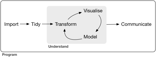
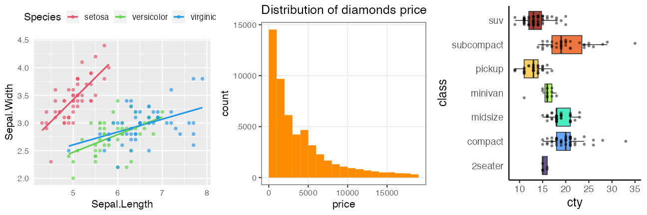
作図してみると全体像・構造が見やすい

情報の整理 → 正しい解析・新しい発見・仮説生成

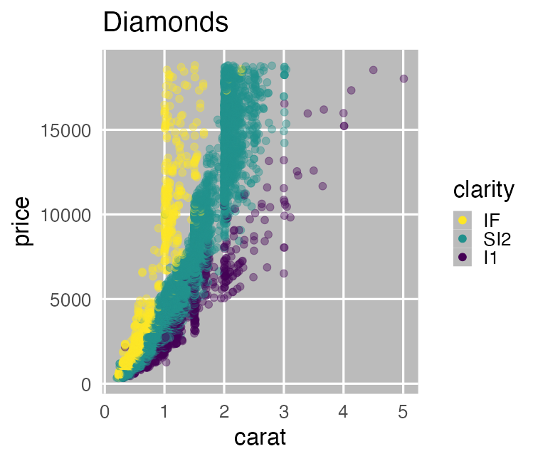
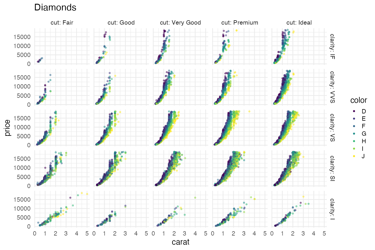
carat が大きいほど price も高いらしい。
その度合いは clarity によって異なるらしい。

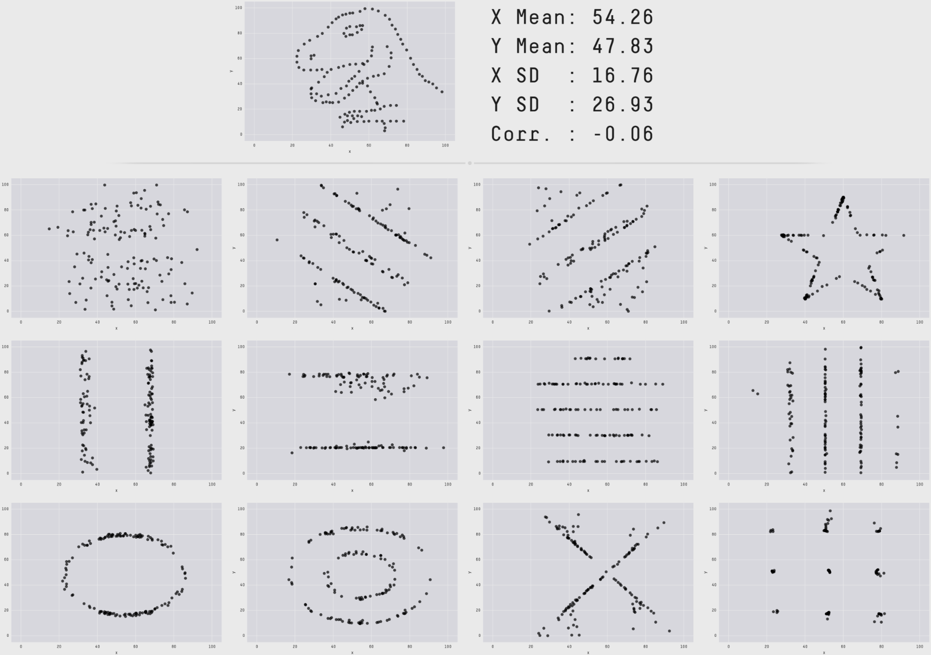
代表値ばかり見て可視化を怠ると構造を見逃す

そうは言ってもセンスでしょ? — NO!

ある程度はテクニックであり教養。
デザインの基本的なルールを
知りさえすれば誰でも上達する。

おしながき: Rによるデータ可視化とレポート作成

✅ データ解析全体の流れ。可視化だいじ

⬜ 一貫性のある文法で合理的に描けるggplot2

⬜ Rのコードと実行結果をレポートに埋め込むQuarto

iris: アヤメ属3種150個体の測定データ

Rに最初から入ってて、例としてよく使われる。

print(iris)

    Sepal.Length Sepal.Width Petal.Length Petal.Width   Species
  1          5.1         3.5          1.4         0.2    setosa
  2          4.9         3.0          1.4         0.2    setosa
  3          4.7         3.2          1.3         0.2    setosa
  4          4.6         3.1          1.5         0.2    setosa
 --                                                            
147          6.3         2.5          5.0         1.9 virginica
148          6.5         3.0          5.2         2.0 virginica
149          6.2         3.4          5.4         2.3 virginica
150          5.9         3.0          5.1         1.8 virginica

長さ150の数値ベクトル4本と因子ベクトル1本。

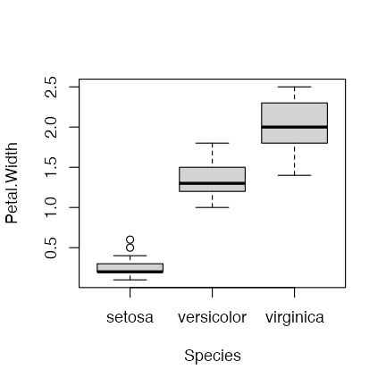
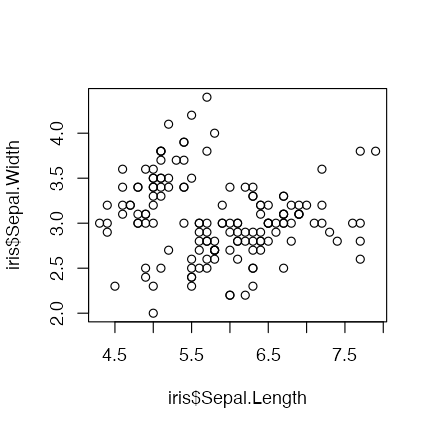
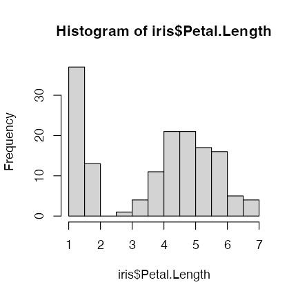
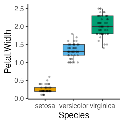
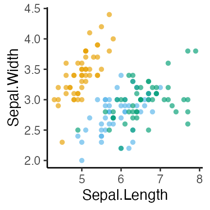
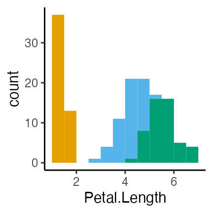
R標準のグラフィックス

描けるっちゃ描けるけど。カスタマイズしていくのは難しい。

boxplot(Petal.Width ~ Species, data = iris)
plot(iris$Sepal.Length, iris$Sepal.Width)
hist(iris$Petal.Length)

きれいなグラフを簡単に描けるパッケージを使いたい。

ggplot2: tidyverseの可視化担当

• “The Grammer of Graphics” という体系に基づく設計
• 単にいろんなグラフを「描ける」だけじゃなく
  一貫性のある文法で合理的に描ける

ggplot2: tidyverseの可視化担当

• “The Grammer of Graphics” という体系に基づく設計
• 単にいろんなグラフを「描ける」だけじゃなく
  一貫性のある文法で合理的に描ける

いきなりggplot2から使い始めても大丈夫

R標準のやつとは根本的に違うシステムで作図する。

基本的な使い方: 指示を + で重ねていく

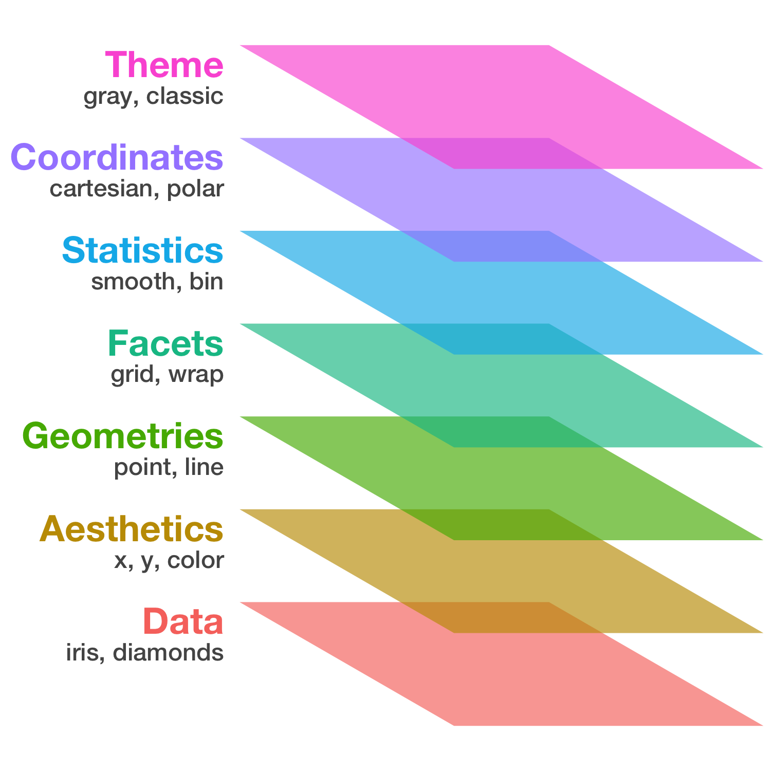
基本的な使い方: 指示を + で重ねていく

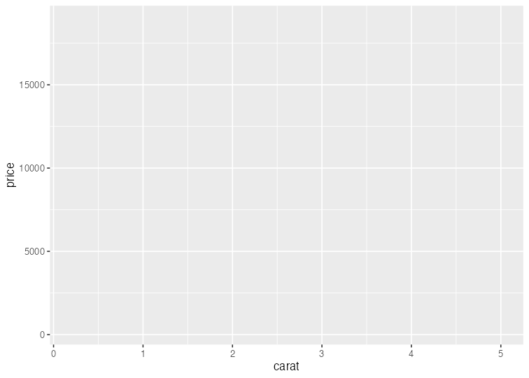
ggplot(data = diamonds)             # diamondsデータでキャンバス準備
# aes(x = carat, y = price) +       # carat,price列をx,y軸にmapping
# geom_point() +                    # 散布図を描く
# facet_wrap(vars(clarity)) +       # clarity列に応じてパネル分割
# stat_smooth(method = lm) +        # 直線回帰を追加
# coord_cartesian(ylim = c(0, 2e4)) + # y軸の表示範囲を狭く
# theme_classic(base_size = 20)     # クラシックなテーマで

基本的な使い方: 指示を + で重ねていく

ggplot(data = diamonds) +           # diamondsデータでキャンバス準備
  aes(x = carat, y = price)         # carat,price列をx,y軸にmapping
# geom_point() +                    # 散布図を描く
# facet_wrap(vars(clarity)) +       # clarity列に応じてパネル分割
# stat_smooth(method = lm) +        # 直線回帰を追加
# coord_cartesian(ylim = c(0, 2e4)) + # y軸の表示範囲を狭く
# theme_classic(base_size = 20)     # クラシックなテーマで

基本的な使い方: 指示を + で重ねていく

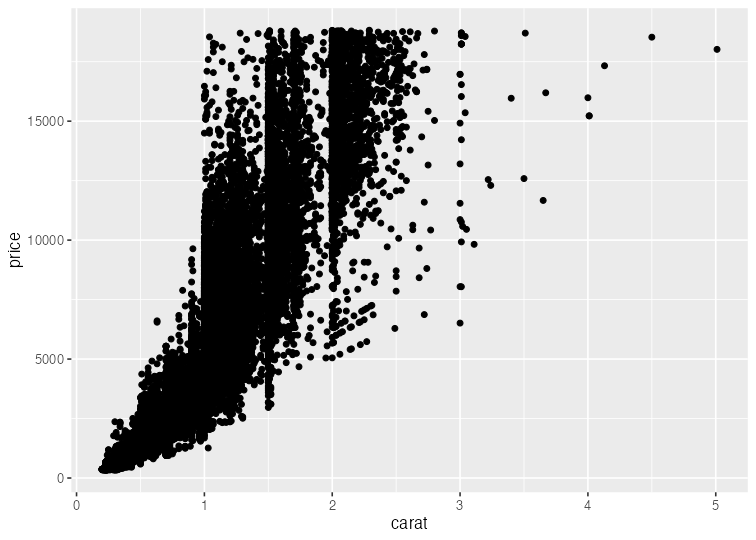
ggplot(data = diamonds) +           # diamondsデータでキャンバス準備
  aes(x = carat, y = price) +       # carat,price列をx,y軸にmapping
  geom_point()                      # 散布図を描く
# facet_wrap(vars(clarity)) +       # clarity列に応じてパネル分割
# stat_smooth(method = lm) +        # 直線回帰を追加
# coord_cartesian(ylim = c(0, 2e4)) + # y軸の表示範囲を狭く
# theme_classic(base_size = 20)     # クラシックなテーマで

基本的な使い方: 指示を + で重ねていく

ggplot(data = diamonds) +           # diamondsデータでキャンバス準備
  aes(x = carat, y = price) +       # carat,price列をx,y軸にmapping
  geom_point() +                    # 散布図を描く
  facet_wrap(vars(clarity))         # clarity列に応じてパネル分割
# stat_smooth(method = lm) +        # 直線回帰を追加
# coord_cartesian(ylim = c(0, 2e4)) + # y軸の表示範囲を狭く
# theme_classic(base_size = 20)     # クラシックなテーマで

基本的な使い方: 指示を + で重ねていく

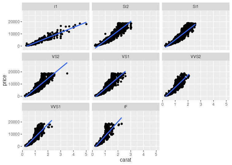
ggplot(data = diamonds) +           # diamondsデータでキャンバス準備
  aes(x = carat, y = price) +       # carat,price列をx,y軸にmapping
  geom_point() +                    # 散布図を描く
  facet_wrap(vars(clarity)) +       # clarity列に応じてパネル分割
  stat_smooth(method = lm)          # 直線回帰を追加
# coord_cartesian(ylim = c(0, 2e4)) + # y軸の表示範囲を狭く
# theme_classic(base_size = 20)     # クラシックなテーマで

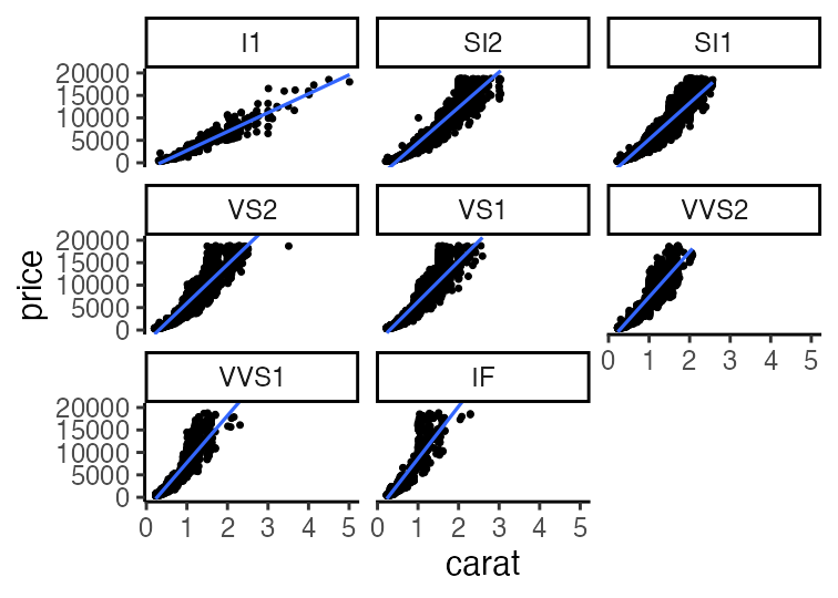
基本的な使い方: 指示を + で重ねていく

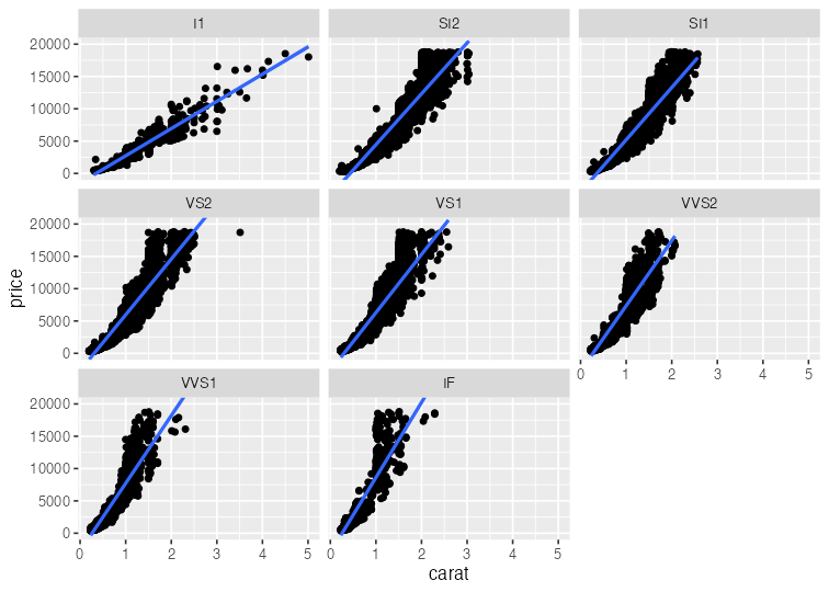
ggplot(data = diamonds) +           # diamondsデータでキャンバス準備
  aes(x = carat, y = price) +       # carat,price列をx,y軸にmapping
  geom_point() +                    # 散布図を描く
  facet_wrap(vars(clarity)) +       # clarity列に応じてパネル分割
  stat_smooth(method = lm) +        # 直線回帰を追加
  coord_cartesian(ylim = c(0, 2e4))   # y軸の表示範囲を狭く
# theme_classic(base_size = 20)     # クラシックなテーマで

基本的な使い方: 指示を + で重ねていく

ggplot(data = diamonds) +           # diamondsデータでキャンバス準備
  aes(x = carat, y = price) +       # carat,price列をx,y軸にmapping
  geom_point() +                    # 散布図を描く
  facet_wrap(vars(clarity)) +       # clarity列に応じてパネル分割
  stat_smooth(method = lm) +        # 直線回帰を追加
  coord_cartesian(ylim = c(0, 2e4)) + # y軸の表示範囲を狭く
  theme_classic(base_size = 20)     # クラシックなテーマで

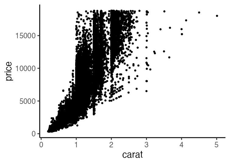
基本的な使い方: 指示を + で重ねていく

ggplot(data = diamonds) +           # diamondsデータでキャンバス準備
  aes(x = carat, y = price) +       # carat,price列をx,y軸にmapping
  geom_point() +                    # 散布図を描く
# facet_wrap(vars(clarity)) +       # clarity列に応じてパネル分割
# stat_smooth(method = lm) +        # 直線回帰を追加
# coord_cartesian(ylim = c(0, 2e4)) + # y軸の表示範囲を狭く
  theme_classic(base_size = 20)     # クラシックなテーマで

途中経過オブジェクトを取っておける

p1 = ggplot(data = diamonds)
p2 = p1 + aes(x = carat, y = price)
p3 = p2 + geom_point()
p4 = p3 + facet_wrap(vars(clarity))
print(p3)

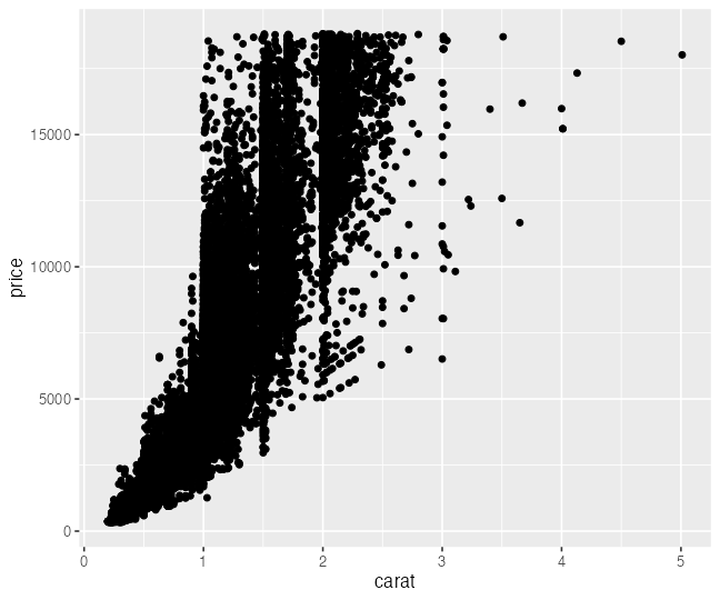
この p3 は後で使います。

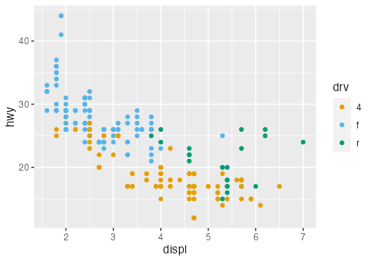
ひとまずggplotしてみよう

自動車のスペックに関するデータ mpg を使って。

    manufacturer  model displ year cyl      trans drv cty hwy fl   class
  1         audi     a4   1.8 1999   4   auto(l5)   f  18  29  p compact
  2         audi     a4   1.8 1999   4 manual(m5)   f  21  29  p compact
 --                                                                     
233   volkswagen passat   2.8 1999   6 manual(m5)   f  18  26  p midsize
234   volkswagen passat   3.6 2008   6   auto(s6)   f  17  26  p midsize

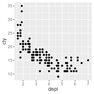
🔰 排気量 displ と市街地燃費 cty の関係を散布図で。

よくあるエラー

関数名を ggplot2 と書いちゃうと勘違い:

> ggplot2(diamonds)
Error in ggplot2(diamonds) : could not find function "ggplot2"

ggplot2 はパッケージ名。
今度こそ関数名は合ってるはずなのに…

> ggplot(diamonds)
Error in ggplot(diamonds) : could not find function "ggplot"

パッケージ読み込みを忘れてた。新しくRを起動するたびに必要:

library(conflicted) # 安全のおまじない
library(tidyverse)  # including ggplot2
ggplot(diamonds)    # OK!

そのほか よくあるエラー集 (石川由希さん@名古屋大) を参照。

ggplot() に渡すのは整然データ tidy data

• 1行は1つの観測
• 1列は1つの変数
• 1セルは1つの値
• この列をX軸、この列をY軸、この列で色わけ、と指定できる！

print(diamonds)

      carat       cut color clarity depth table price    x    y    z
    1  0.23     Ideal     E     SI2  61.5    55   326 3.95 3.98 2.43
    2  0.21   Premium     E     SI1  59.8    61   326 3.89 3.84 2.31
    3  0.23      Good     E     VS1  56.9    65   327 4.05 4.07 2.31
    4  0.29   Premium     I     VS2  62.4    58   334 4.20 4.23 2.63
   --                                                               
53937  0.72      Good     D     SI1  63.1    55  2757 5.69 5.75 3.61
53938  0.70 Very Good     D     SI1  62.8    60  2757 5.66 5.68 3.56
53939  0.86   Premium     H     SI2  61.0    58  2757 6.15 6.12 3.74
53940  0.75     Ideal     D     SI2  62.2    55  2757 5.83 5.87 3.64

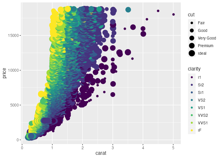
Aesthetic mapping でデータと見せ方を紐付け

aes() の中で列名を指定する。

ggplot(diamonds) +
  aes(x = carat, y = price) +
  geom_point(mapping = aes(color = clarity, size = cut))

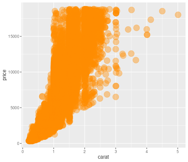
データによらず一律でaestheticsを変える

aes() の外で値を指定する。

ggplot(diamonds) +
  aes(x = carat, y = price) +
  geom_point(color = "darkorange", size = 6, alpha = 0.4)

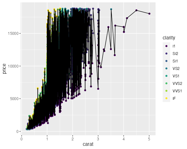
外の aes() は全ての geom_*() に波及する

ggplot(diamonds) +
  aes(x = carat, y = price) +
  geom_point(aes(color = clarity)) +
  geom_line()             # NO color
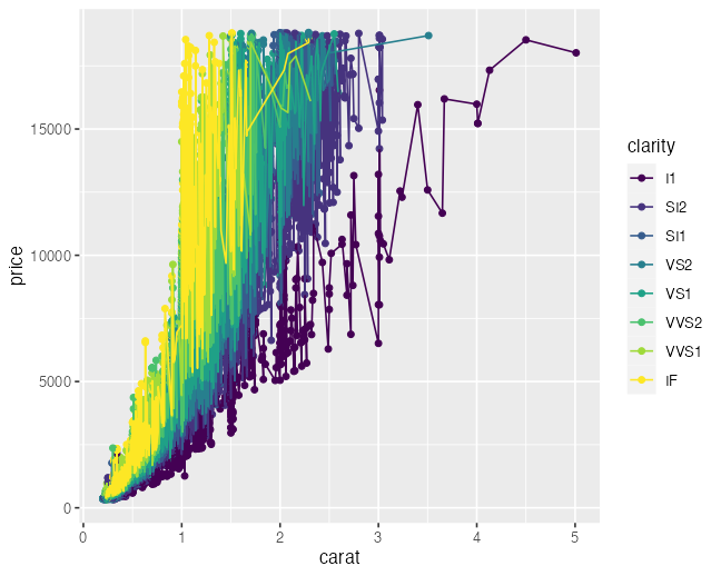
ggplot(diamonds) +
  aes(x = carat, y = price, color = clarity) +
  geom_point() +          # color
  geom_line()             # color

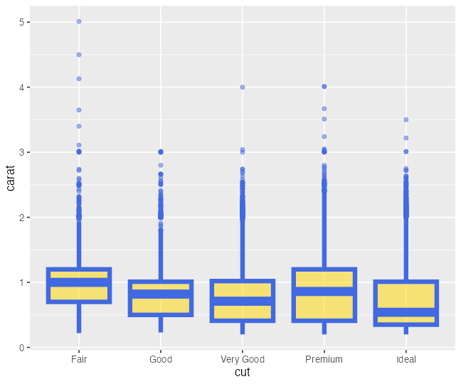
aesthetics一覧

• 色・透明度を変える
  • color: 点、線、文字の色
  • fill: 面の色
  • alpha: 不透明度 (0が透明、1が不透明)
• 大きさ・形を変える
  • size, shape: 点の大きさや形
  • linewidth, linetype: 線の太さや種類
• 単にグループ分けする
  • group: 折れ線グラフやポリゴンの切り分けなど
• 座標、始点、終点
  • x, y, xmin, xmax, ymin, ymax, xend, yend

点と線と文字は color, 面は fill

不透明度は alpha

ggplot(diamonds) +
  aes(cut, carat) +
  geom_boxplot(color = "royalblue", fill = "gold", alpha = 0.5, linewidth = 2)

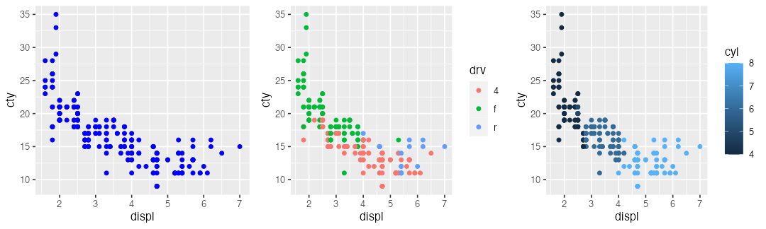
色の変え方の練習

自動車のスペックに関するデータ mpg を使って。

    manufacturer  model displ year cyl      trans drv cty hwy fl   class
  1         audi     a4   1.8 1999   4   auto(l5)   f  18  29  p compact
  2         audi     a4   1.8 1999   4 manual(m5)   f  21  29  p compact
 --                                                                     
233   volkswagen passat   2.8 1999   6 manual(m5)   f  18  26  p midsize
234   volkswagen passat   3.6 2008   6   auto(s6)   f  17  26  p midsize

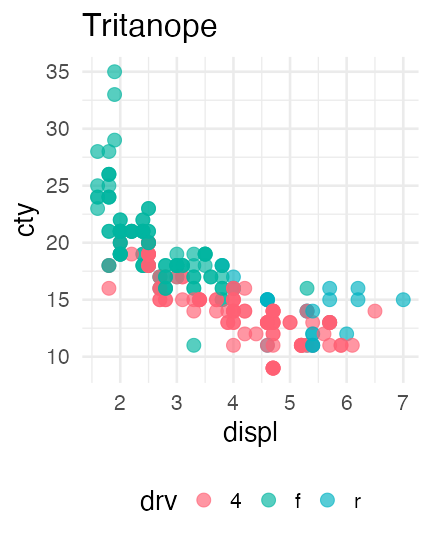
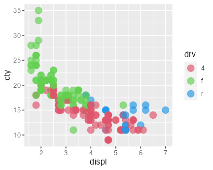
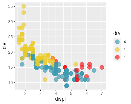
🔰 排気量 displ と市街地燃費 cty の関係を青い散布図で描こう
🔰 駆動方式 drv やシリンダー数 cyl によって色を塗り分けしてみよう

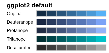
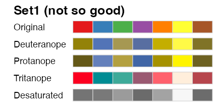
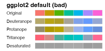
色の見え方は人によって違う

赤 緑 青の3色を使った先ほどの図は多くの人には問題なさそう。
しかし5%くらいの人には右のように赤 緑 青 や 赤 緑 青の2色に見えている。

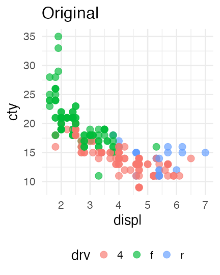
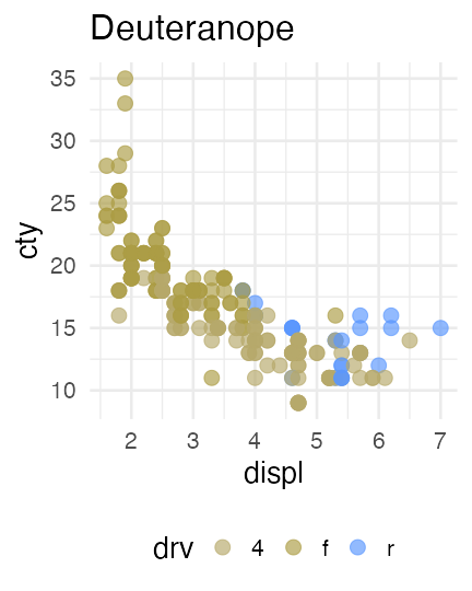
MacやiOSならSim Daltonismというアプリでシミュレーションできる。
WindowsならColor Oracleが使えそう。

多様性を前提によく考えられたパレットもある

Sequential palette:

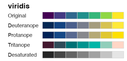
Diverging palette:

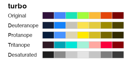
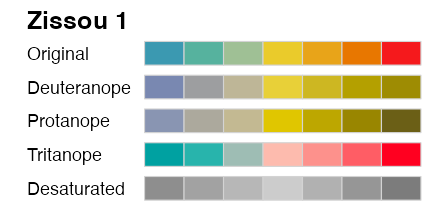
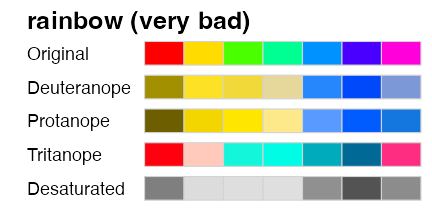
Qualitative (categorical, discrete) palette:

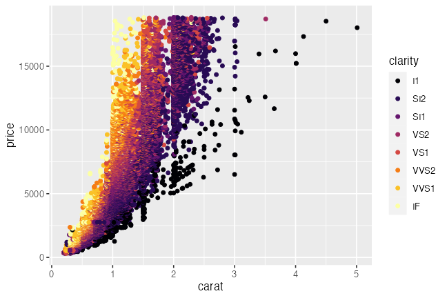
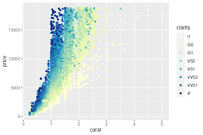
色パレットの変更 scale_color_*()

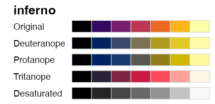
viridis と ColorBrewer のパレットはggplot2に組み込まれているので簡単。
上記リンクから名前を探して、option = か palette = で指定。

ggplot(diamonds) + aes(carat, price) +
  geom_point(mapping = aes(color = clarity)) +
  scale_color_viridis_d(option = "inferno")
# scale_color_brewer(palette = "YlGnBu")

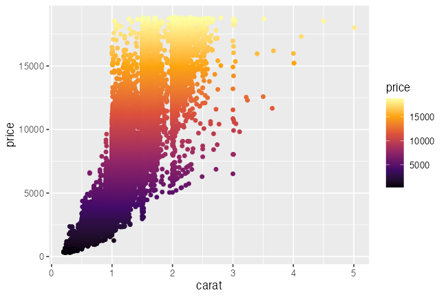
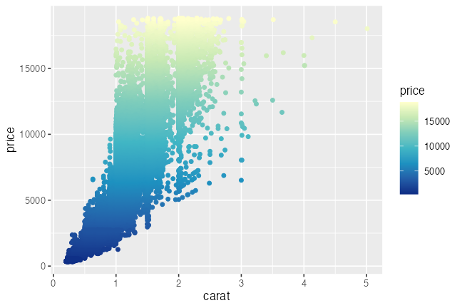
連続値(continuous)と離散値(discrete)を区別する

渡す値とscale関数が合ってないと怒られる:
Error: Continuous value supplied to discrete scale

ggplot(diamonds) + aes(carat, price) +
  geom_point(mapping = aes(color = price)) +
  scale_color_viridis_c(option = "inferno")
# scale_color_distiller(palette = "YlGnBu")

• discrete: scale_color_viridis_d(), scale_color_brewer()
• continuous: scale_color_viridis_c(), scale_color_distiller()
• binned: scale_color_viridis_b(), scale_color_fermenter()

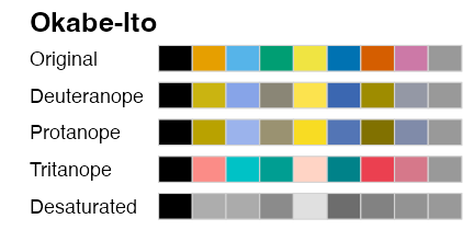
viridisやbrewer以外のパレットを使うには

R標準の palette.colors() や colorspaceパッケージ を使う。

okabe_ito = palette.colors(9L, "Okabe-Ito")
ggplot(mpg) +
  aes(x = displ, y = cty) +
  geom_point(aes(color = drv), size = 4, alpha = 0.66) +
  scale_color_discrete(type = unname(okabe_ito)[-1])
# scale_color_discrete(type = palette.colors(8L, "R4")[-1])
# colorspace::scale_colour_discrete_divergingx("Zissou 1")

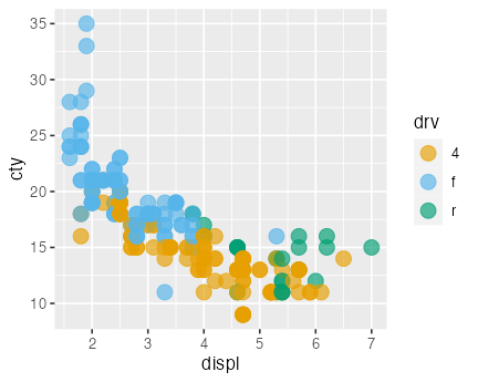
自分で全色個別指定もできるが、専門家の考えたセットを使うのが無難。

scale_color_* を省略できるように設定することも可能

連続値viridis, 離散値Okabe-Itoをデフォルトにする例:

grDevices::palette("Okabe-Ito")
options(
  ggplot2.continuous.colour = "viridis",
  ggplot2.continuous.fill = "viridis",
  ggplot2.discrete.colour = grDevices::palette()[-1],
  ggplot2.discrete.fill = grDevices::palette()[-1]
)

options() による設定はRを終了するまで有効。

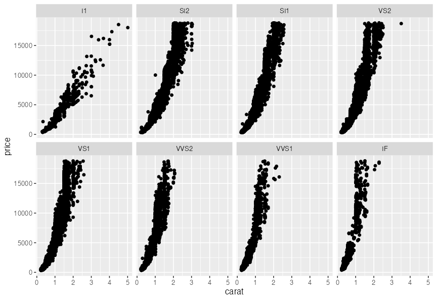
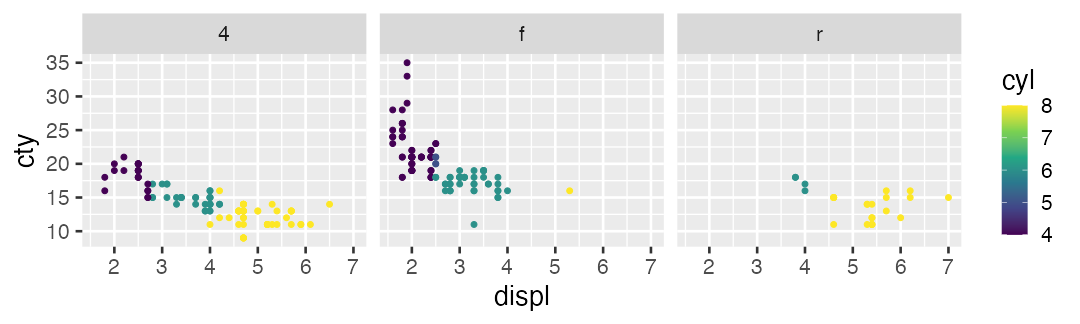
値に応じてパネル切り分け (1変数facet)

ggplotの真骨頂！ これをR標準機能でやるのは結構たいへん。

p3 + facet_wrap(vars(clarity), ncol = 4L)

値に応じてパネル切り分け (≥2変数facet)

ggplotの真骨頂！ これをR標準機能でやるのは結構たいへん。

p3 + facet_grid(vars(clarity), vars(cut))

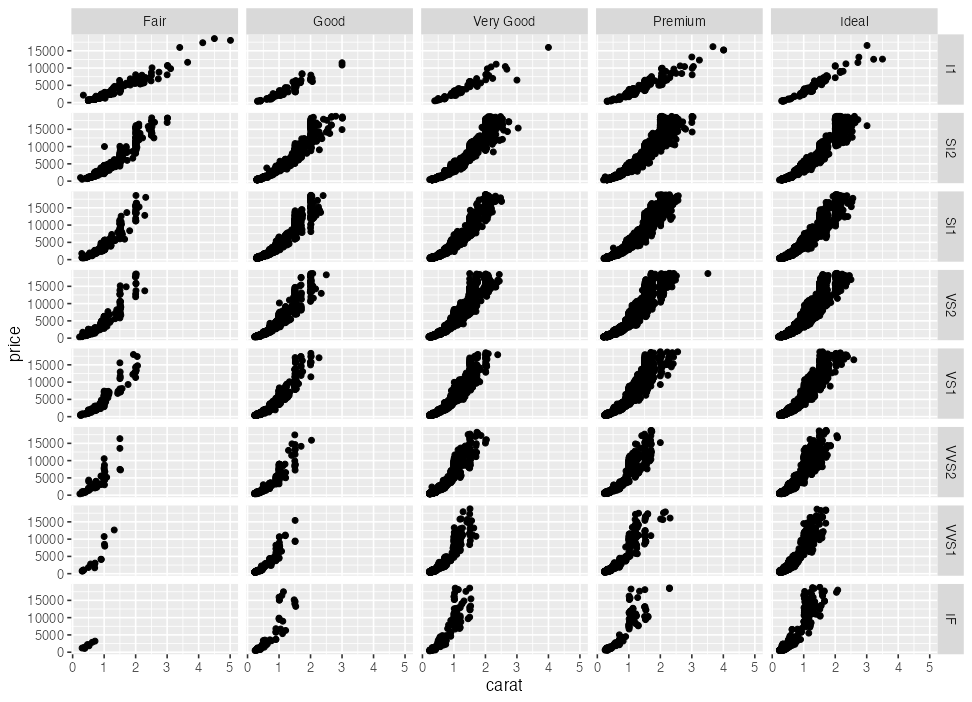
多変量データの俯瞰、5次元くらいまで有効

値に応じたfacetの練習

自動車のスペックに関するデータ mpg を使って。

    manufacturer  model displ year cyl      trans drv cty hwy fl   class
  1         audi     a4   1.8 1999   4   auto(l5)   f  18  29  p compact
  2         audi     a4   1.8 1999   4 manual(m5)   f  21  29  p compact
 --                                                                     
233   volkswagen passat   2.8 1999   6 manual(m5)   f  18  26  p midsize
234   volkswagen passat   3.6 2008   6   auto(s6)   f  17  26  p midsize

🔰 駆動方式 drv やシリンダー数 cyl によってfacetしてみよう

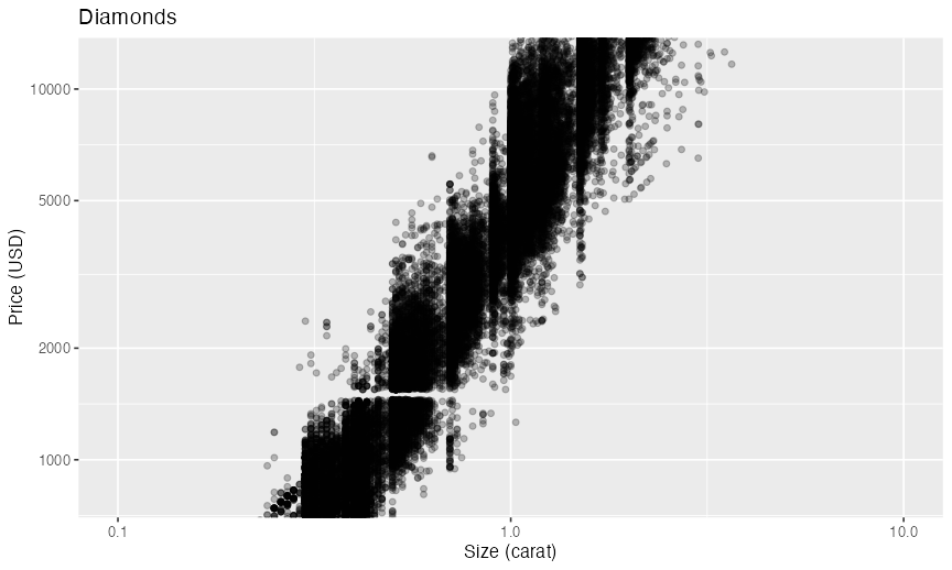
値を変えず座標軸を変える scale_*, coord_*

ggplot(diamonds) + aes(carat, price) + geom_point(alpha = 0.25) +
  scale_x_log10() +
  scale_y_log10(breaks = c(1, 2, 5, 10) * 1000) +
  coord_cartesian(xlim = c(0.1, 10), ylim = c(800, 12000)) +
  labs(title = "Diamonds", x = "Size (carat)", y = "Price (USD)")

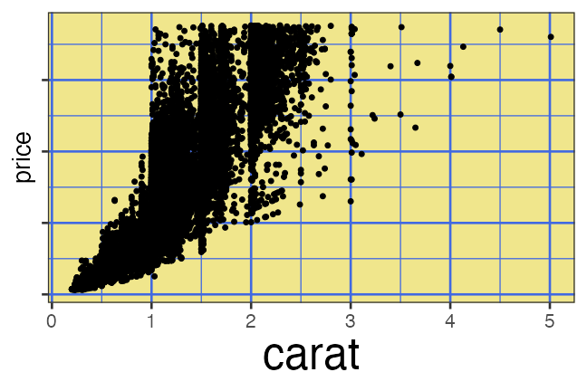
データと関係ない部分の見た目を調整 theme

既存の theme_*() をベースに、theme()関数で微調整。

p3 + theme_bw(base_size = 18) + theme(
  panel.background = element_rect(fill = "khaki"),      # 箱
  panel.grid       = element_line(color = "royalblue"), # 線
  axis.title.x     = element_text(size = 32),           # 文字
  axis.text.y      = element_blank()                    # 消す
)

基本的な使い方: 指示を + で重ねていく

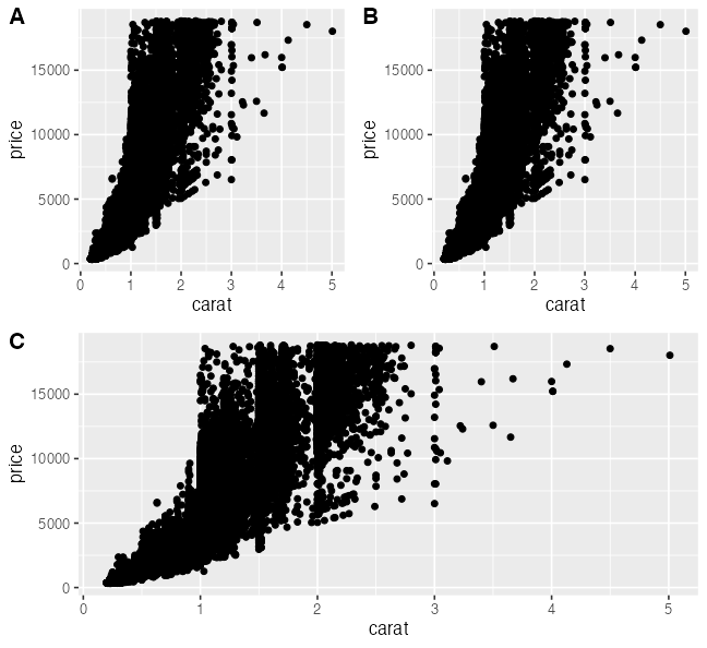
論文のFigureみたいに並べる

別のパッケージ (cowplot や patchwork) の助けを借りて

pAB = cowplot::plot_grid(p3, p3, labels = c("A", "B"), nrow = 1L)
cowplot::plot_grid(pAB, p3, labels = c("", "C"), ncol = 1L)

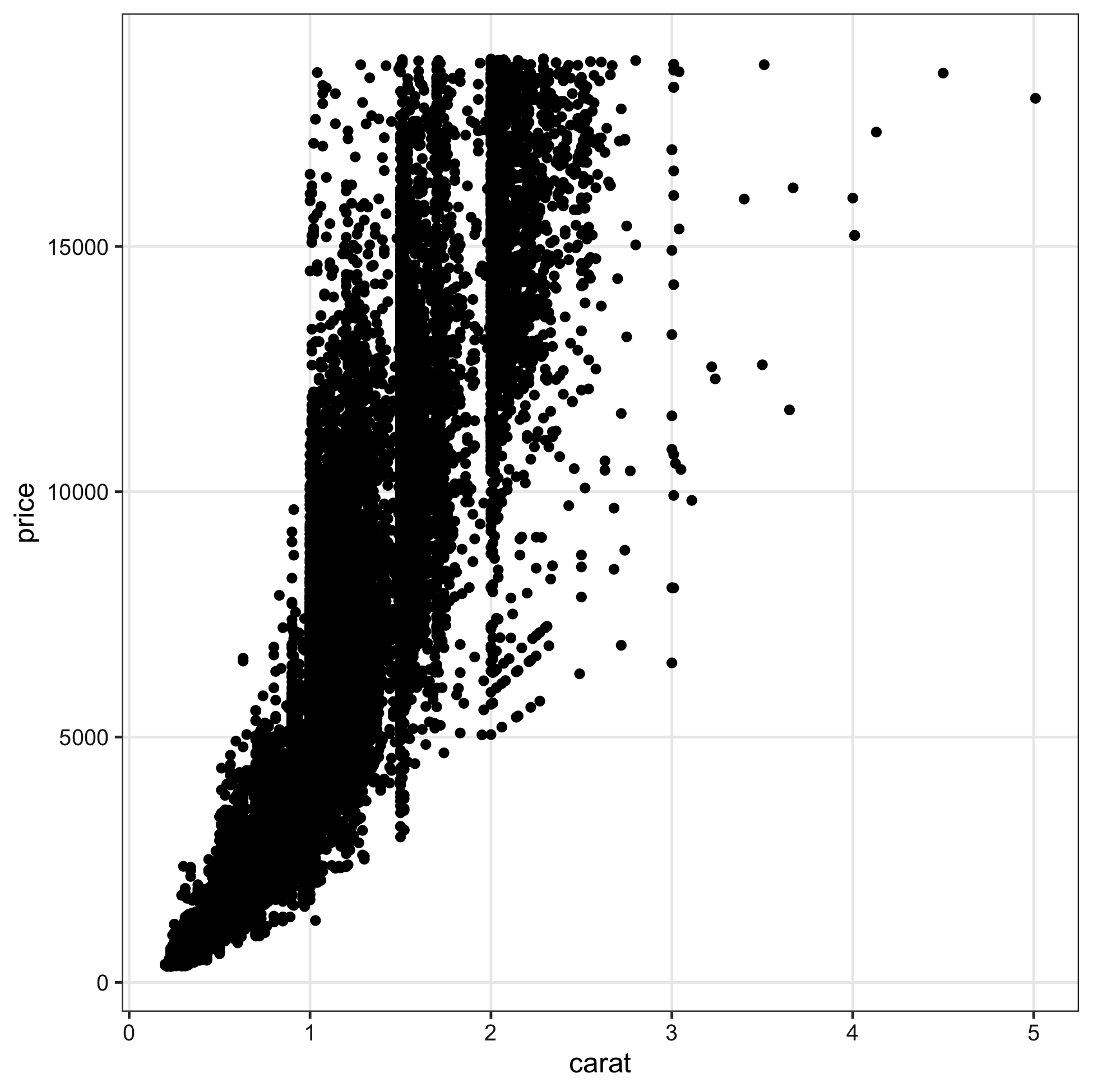
ファイル名もサイズも再現可能な作図

widthやheightが小さいほど、文字・点・線が相対的に大きく

# 7inch x 300dpi = 2100px四方 (デフォルト)
ggsave("dia1.png", p3) # width = 7, height = 7, dpi = 300
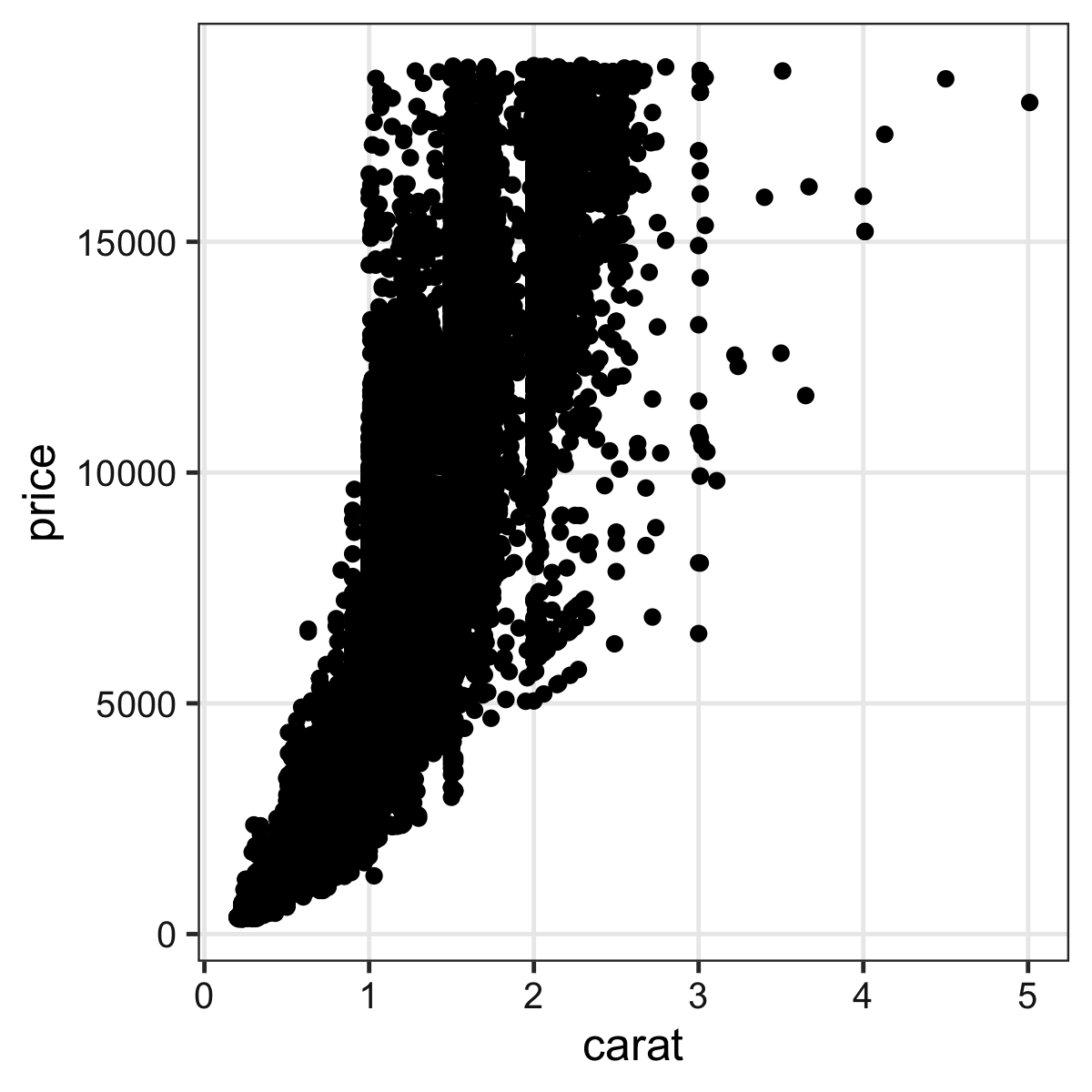
# 4     x 300    = 1200  全体7/4倍ズーム
ggsave("dia2.png", p3, width = 4, height = 4) # dpi = 300
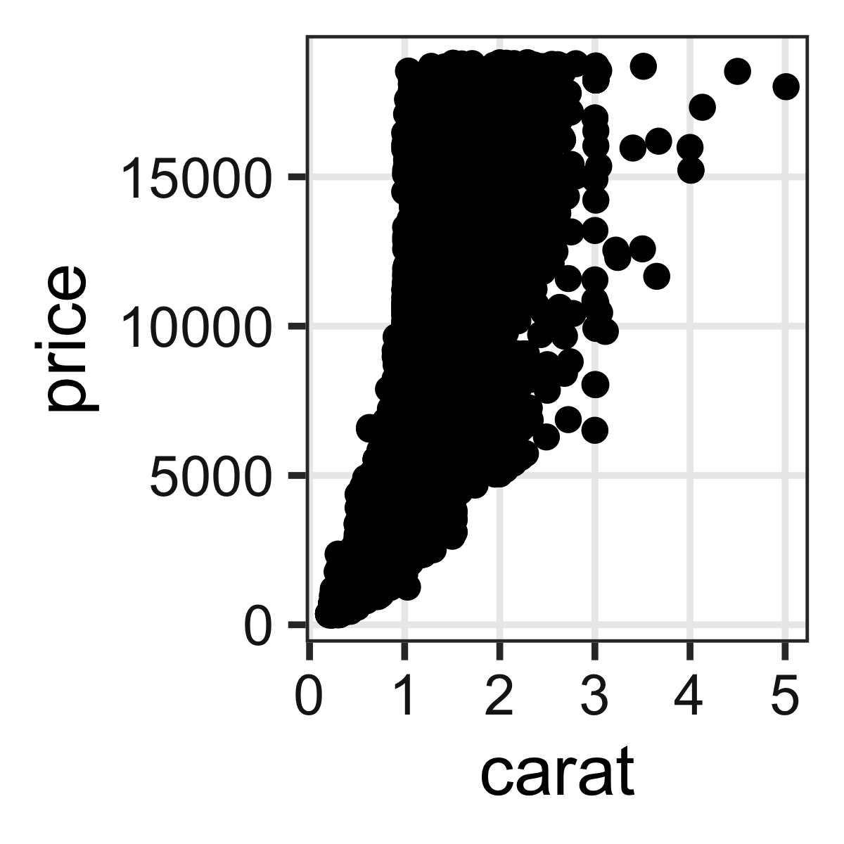
# 2     x 600    = 1200  全体をさらに2倍ズーム
ggsave("dia3.png", p3, width = 2, height = 2, dpi = 600)
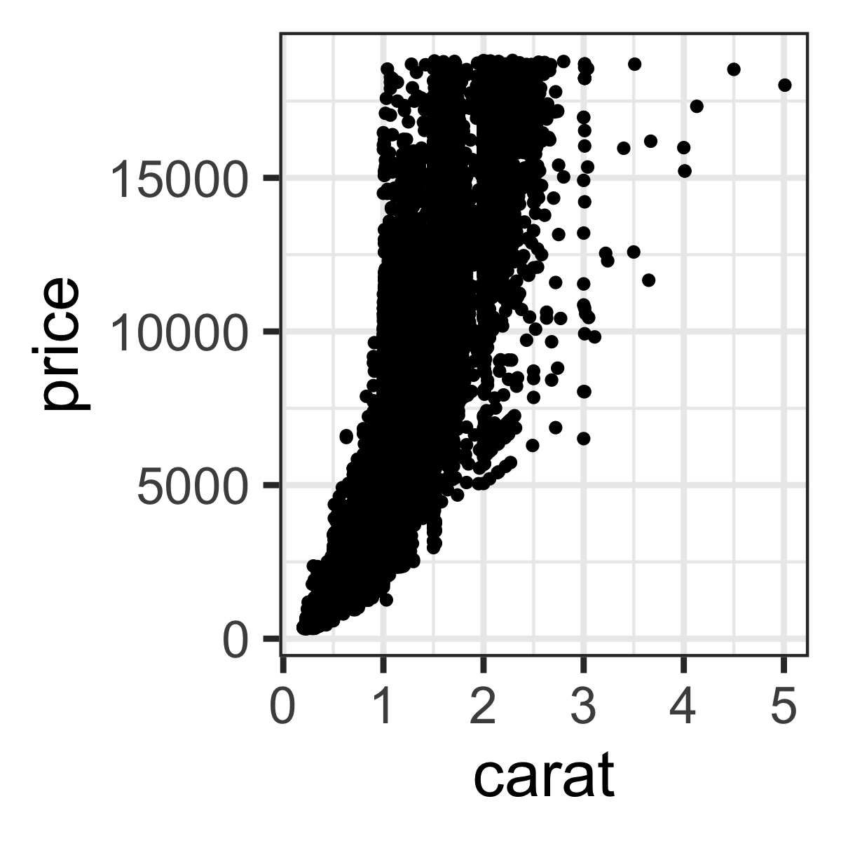
# 4     x 300    = 1200  テーマを使って文字だけ拡大
ggsave("dia4.png", p3 + theme_bw(base_size = 22), width = 4, height = 4)

日本語が◻️◻️◻️豆腐にならないための設定

環境設定 → General → Graphics → Backend: AGG

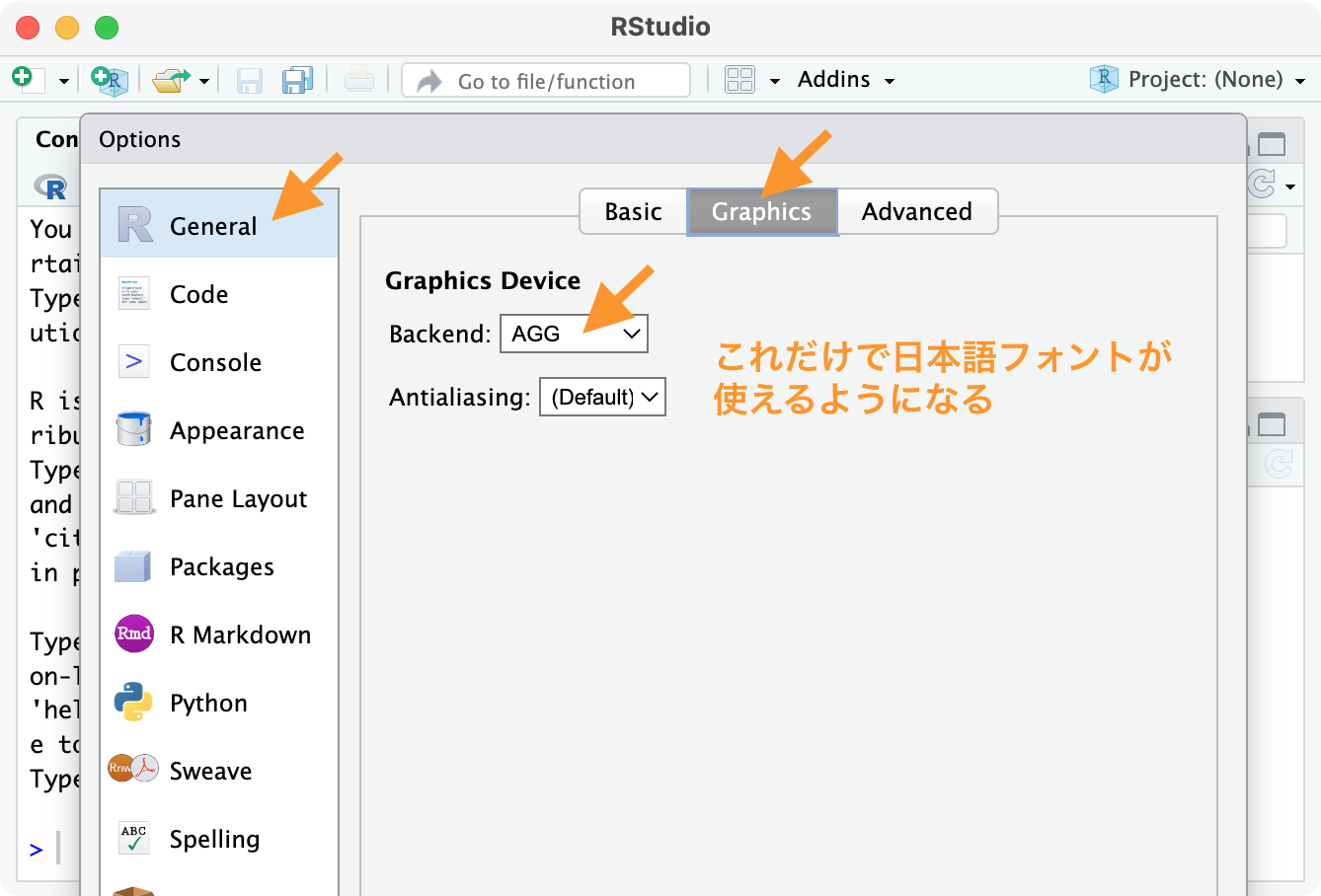
英数字以外を使わずに済ませられればそれに越したことはないけど…

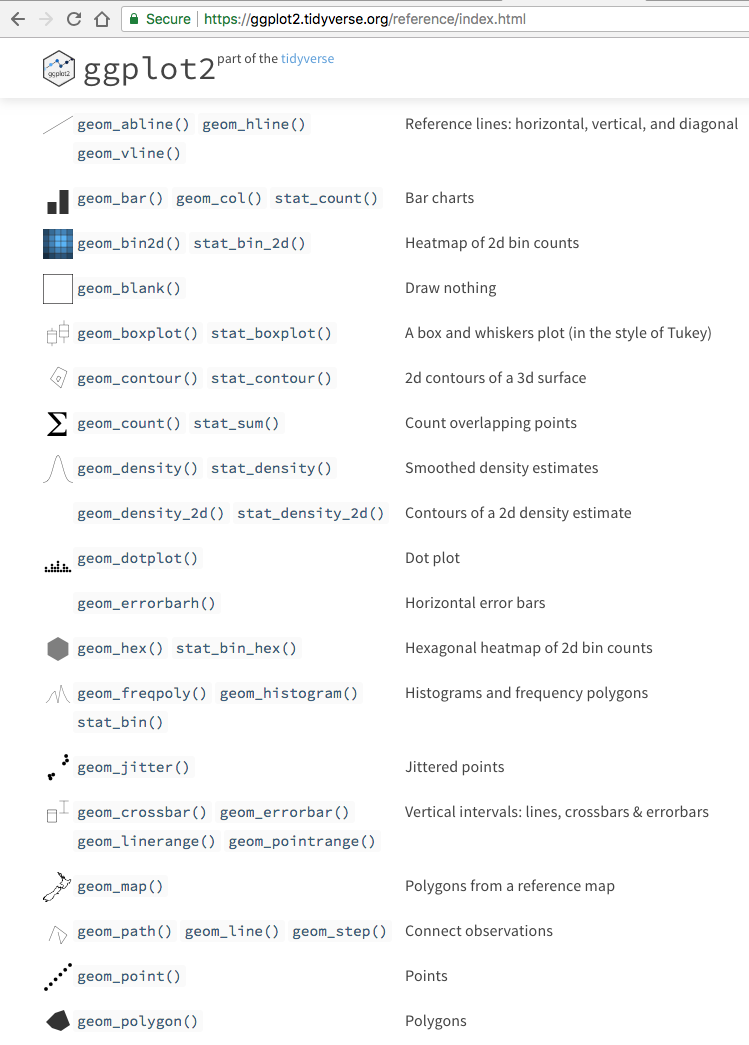
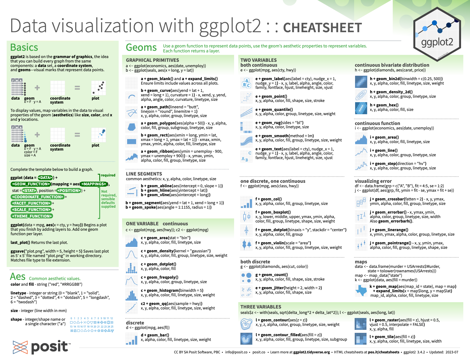
他にどんな種類の geom_*() が使える？

なんでもある。 公式サイトを見に行こう。

微調整してくと最終的に長いコードになるね…

うん。でもすべての点について後から確認できるし、使い回せる！

set.seed(1)
p = ggplot(diamonds) +
  aes(x = cut, y = price) +
  geom_jitter(aes(color = cut), height = 0, width = 0.2, alpha = 0.1, stroke = 0) +
  geom_boxplot(fill = NA, outlier.shape = NA) +
  scale_color_viridis_d(option = "plasma") +
  facet_wrap(vars(clarity)) +
  coord_flip(xlim = c(0.5, 5.5), ylim = c(0, 20000), expand = FALSE) +
  labs(title = "Diamonds", x = "Cut", y = "Price (USD)") +
  theme_bw(base_size = 20) +
  theme(legend.position = "none",
        axis.ticks = element_blank(),
        panel.grid.major.y = element_blank(),
        panel.spacing.x = grid::unit(3, "lines"),
        plot.margin = grid::unit(c(1, 2, 0.5, 0.5), "lines"))
print(p)
ggsave("diamonds-cut-price.png", p, width = 12, height = 9)

発展的な内容

ggplot2をさらに拡張するパッケージも続々

アニメーション gganimate

重なりを避けてラベル付け ggrepel

グラフ/ネットワーク ggraph

系統樹 ggtree

地図 geom_sf

学術論文向けのいろいろ ggpubr

ggplot2は3Dが苦手

本当に3Dが必要? 色分けやファセットで足りない?

別のパッケージでやる: rgl, plotly, etc.

🔰 1日目の課題1: 模写

下図になるべく似るように作図・調整してください。

• 細かい設定まで見逃さないように、班で協力しましょう。

🔰 1日目の課題2: 未登場の関数・オプションを紹介

1. ggplot2に関して本講義で説明されなかった関数やオプションを探す。
   公式サイトや解説ブログなどを参考に。
2. それを使って、作図してみる。
3. 「この講義を受けてggplot2の基礎はわかった」くらいの友達に紹介するつもりで、 使い方の説明をレポートに書く。 どういうときに使えそうか、が説明できるとなお良い。

説明文、Rコード、実行結果、図。
それらをひとまとめに扱えるようなシステムがあるらしい…

おしながき: Rによるデータ可視化とレポート作成

✅ データ解析全体の流れ。可視化だいじ

✅一貫性のある文法で合理的に描けるggplot2

• aesthetic mapping が鍵
• 色覚多様性を意識
• 画像出力まできっちりプログラミング

⬜ Rのコードと実行結果をレポートに埋め込むQuarto

Rコードの実行結果をとっておきたい

スクリプト.Rさえ保存しておけばいつでも実行できるけど… 面倒

ggsave() で画像を書き出しておけるけど… どのコードの結果か分からない

→ スクリプトと実行結果を一緒に見渡せる形式が欲しい。

3 * 14
ggplot(mpg) + aes(displ, hwy) + geom_point(aes(color = drv))

[1] 42

Quarto Document として研究ノートを作る

プログラミングからレポート作成まで一元管理できて楽ちん。

• 本文とRコードを含むテキストファイル.qmdを作る。
• HTML, PDFなどリッチな形式に変換して読む。
  • コードだけでなく実行結果の図や表も埋め込める。

Quarto Markdown (.qmd)

Markdown亜種。RやPythonのコードと図表を埋め込める。

Quarto登場前にほぼR専用だった .Rmd と使い勝手は同じ。

Markdown (.md)

最もよく普及している軽量マークアップ言語のひとつ。

微妙に異なる方言がある。qmdで使うのは Pandoc Markdown 。

(どんなものが作れるのか 作成例ギャラリー を見てみよう。)

マークアップ言語

文書の構造や視覚的修飾を記述するための言語。
e.g., HTML+CSS, XML, LaTeX

<h3>見出し3</h3>
<p>ここは段落。
<em>強調(italic)</em>、
<strong>強い強調(bold)</strong>、
<a href="https://www.lifesci.tohoku.ac.jp/">リンク</a>とか。
</p>

表現力豊かで強力だが人間が読み書きするには複雑すぎ、機械寄り。

(好きなウェブサイトのHTMLソースコードを見てみよう。)

軽量マークアップ言語

マークアップ言語の中でも人間が読み書きしやすいもの。
e.g., Markdown, reStructuredText, 各種Wiki記法など

### 見出し3

ここは段落。
*強調(italic)*、
**強い強調(bold)**、
[リンク](https://www.lifesci.tohoku.ac.jp/)とか。

Quartoする環境は既に整っているはず

• R (≥ 4.2.3): 最新版 – 0.1 くらいまでが許容範囲
• RStudio (≥ 2023.03.0+386): Quarto CLI を同梱
• tidyverse (≥ 2.0.0): 次の2つを自動インストール
  • rmarkdown (≥ 2.21)
  • knitr (≥ 1.42)

(示してあるバージョンは最低要件ではなく私の現在の環境の)

• Quarto CLI: 最新版を求めるなら手動で入れる。
• install.packages("quarto"): 多くの人には不要。 Quarto CLIをRコマンドで呼べるようにするだけ。
• pandoc: Quarto CLI に同梱。 手動で最新版を入れてもRStudio+Quartoがそれを使うかは不明。

Markdown記法で書いてみよう

1. RStudio > New File > Markdown File
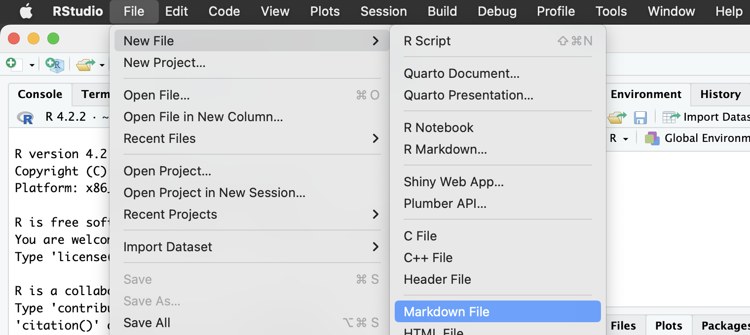
2. “markdown 記法"で検索して何か書く。 最低限、次の概念を含むように:
   • 見出し1, 2, 3
   • コードブロック、インラインコード
   • 箇条書き (番号あり・なし)
3. Previewボタンで確認

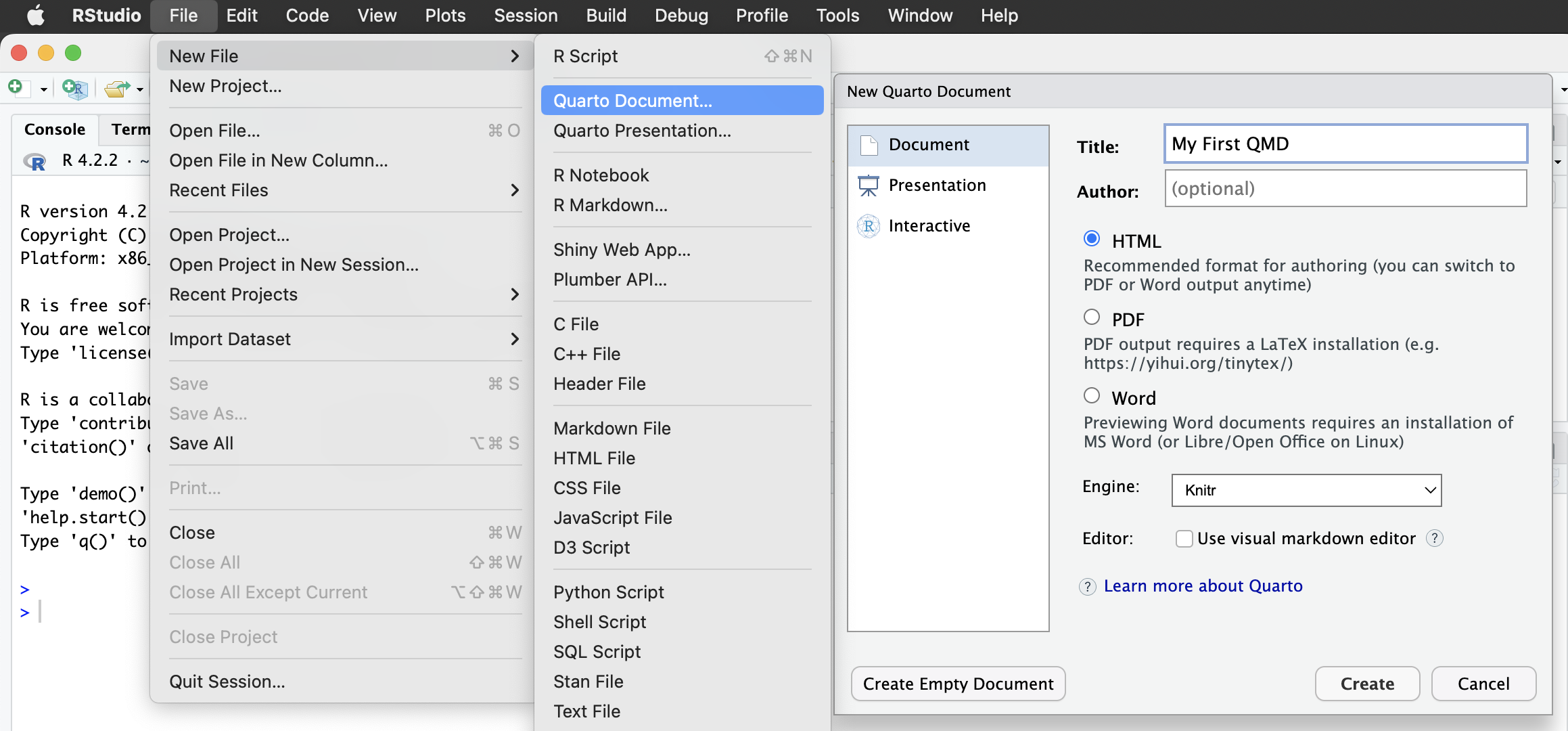
Quarto Document を作ってみよう

RStudio > New File > Quarto Document…
(DocumentとHTMLを選択し、)タイトルと著者を埋めて、OK。

普通のmdには無いqmdの特徴

ヘッダー (フロントマター)

最上部の --- で挟まれた部分。 文書全体に関わるメタデータを入力。

オプションは出力形式によって異なる。 e.g., html

R code chunk

```{r} のように始まるコードブロック。

コードの実行結果を最終産物に埋め込める。

オプションがいろいろある。e.g.,

• echo: false: コードを非表示。結果は表示。
• eval: false: コードを実行せず表示だけ。
• include: false: コードも結果も表示せず、実行だけする。
• fig.width: 7, fig.height: 7: 図の大きさを制御。

まあ細かいことは必要になってから調べるとして…

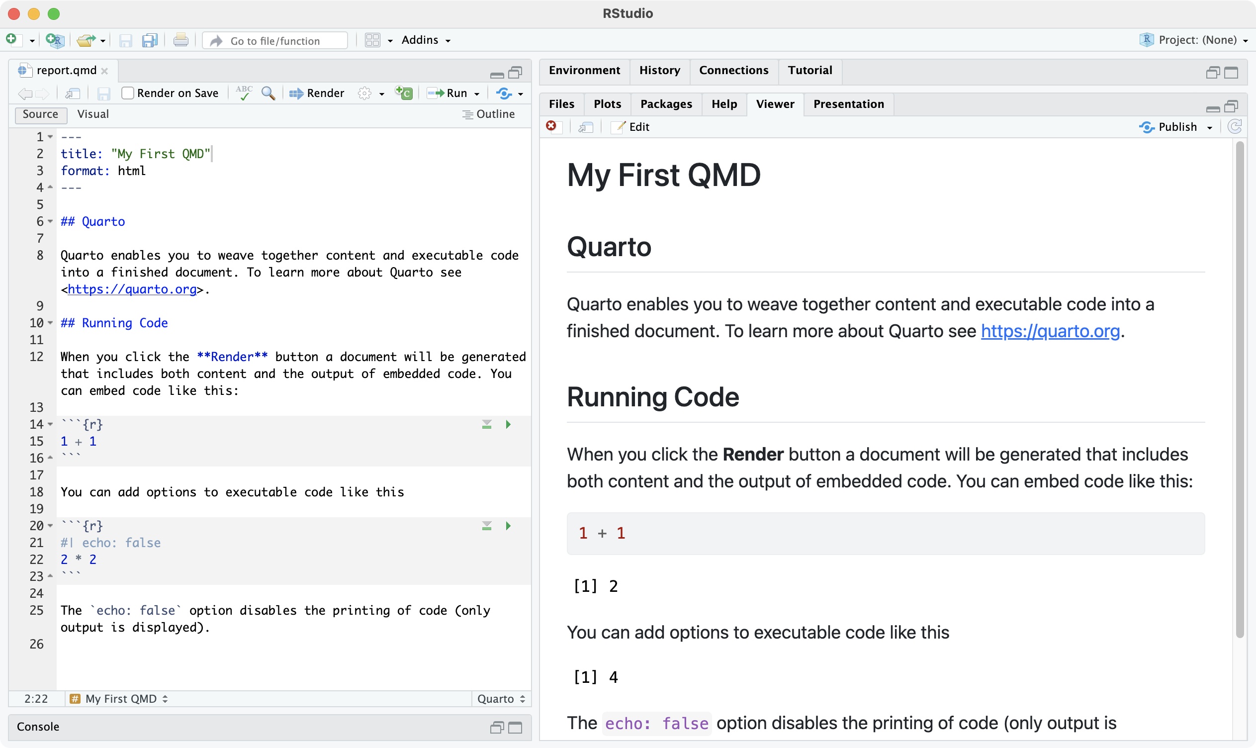
qmdをHTMLに変換してみよう

左のqmdを “→Render” すると右のができる。手順は次スライド。

qmdをHTMLに変換してみよう

1. ソースコードに名前をつけて保存 commands
   e.g., report.qmd
2. ⚙️ ボタンから “Preview in Viewer Pane” を選択。
3. “→Render” を押す。
   • 埋め込まれたRコードが実行される。
   • 実行結果を含むMarkdownが作られる。
   • MarkdownからHTMLに変換される。 e.g., report.html
   • プレビューが自動的に開く。
4. 編集 → 保存 → Render を繰り返して作り込む。

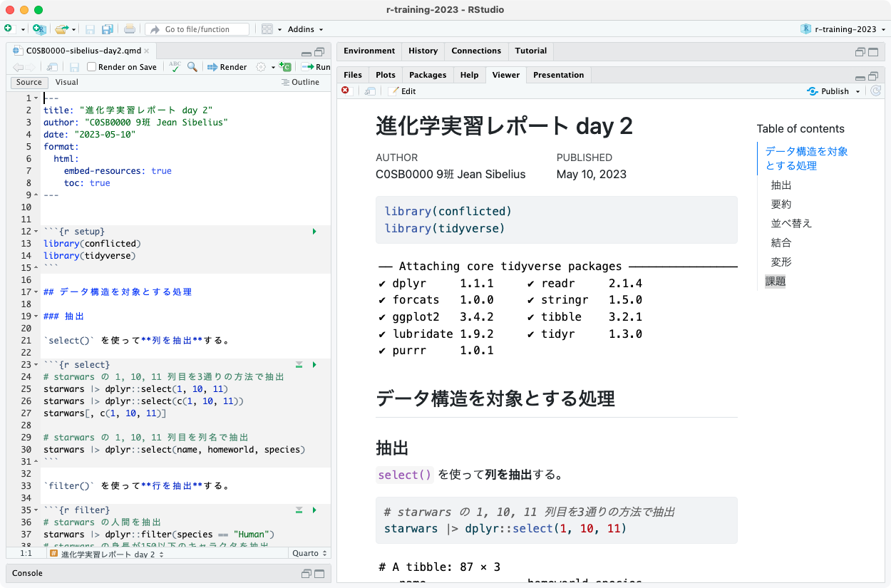
レポートの体裁の例

左のようなqmdを作ってRenderし、右のようなHTMLファイルを提出。

🔰 レポート (締切: 2023-05-18)

• 酒井先生のレポート講座5/8を受けてから提出。
• 課題: 講義資料の🔰若葉マークすべて。
• 様式: Quarto Markdownで書き、Render済みHTMLを提出。
  • 1日分で1ファイル、それぞれClassroomトピックに提出。計4つ。
  • {ID}-{name}-day{d}.html, e.g., C0SB0000-iwasaki-day2.html
  • embed-resources: true で画像などを埋め込んだ独立HTML。
• 評価ポイント
  • エラーも警告も無くコードが走る。
  • 文書の構造や図が視覚的に見やすく整理されている。
  • 半年後の自分が読んでわかるような # 親切コメント。
• 手抜きポイント
  • 生物学的な意義があるか、みたいなのはほぼ不問。

今日の残り時間

• 班やTAに相談し、消化しきれなかった部分をなるべく解消する。
• 課題1 模写を ggsave() まできっちりやる。
• TAが班の代表画像を評価し、合格した班から解散。
• 残ってほかの課題に取り組んでもOK。

参考

R for Data Science — Hadley Wickham and Garrett Grolemund

https://r4ds.had.co.nz/

Book

日本語版書籍(Rではじめるデータサイエンス)

Older versions

「Rにやらせて楽しよう — データの可視化と下ごしらえ」 岩嵜航 2018

「Rを用いたデータ解析の基礎と応用」石川由希 2019 名古屋大学

「Rによるデータ前処理実習」 岩嵜航 2022 東京医科歯科大

「Rを用いたデータ解析の基礎と応用」 石川由希 2022 名古屋大学

ggplot2公式ドキュメント

https://ggplot2.tidyverse.org/