統計モデリング概論 DSHC 2024

1. 導入
2. 直線回帰、確率分布、擬似乱数生成
3. 尤度、最尤推定
4. 一般化線形モデル(GLM)
5. 個体差、一般化線形混合モデル(GLMM)
6. ベイズの定理、事後分布、MCMC
7. StanでGLM
8. 階層ベイズモデル(HBM)

🔰 とりあえずStanを動かしてみよう

This is cmdstanr version 0.8.1
- CmdStanR documentation and vignettes: mc-stan.org/cmdstanr
- CmdStan path: /Users/watal/.cmdstan/cmdstan-2.36.0
- CmdStan version: 2.36.0

This is bayesplot version 1.11.1.9000

おおまかな流れ:

1. データ準備
2. Stan言語でモデルを書く
3. モデルをコンパイルして機械語に翻訳 → 実行ファイル
4. 実行ファイルにデータを渡してMCMCサンプリング
5. 結果を見る

🔰 7-stan.ipynb を開き、スライド説明に沿って実行しよう。

説明変数なしのベイズ推定: データ準備

表が出る確率 $p=0.7$ のイカサマコインをN回投げたデータを作る。
この $p$ をStanで推定してみよう。

true_p = 0.7
N = 40L
coin_data = list(N = N, x = rbinom(N, 1, true_p))
print(coin_data)

$N
[1] 40

$x
 [1] 1 0 0 1 1 1 1 0 1 0 1 1 0 1 1 0 1 1 1 1 0 0 1 1 1 1 1 1 1 0 1 1 0 1 1 0 1 1 1 1

Rならlist型、Pythonならdict型にまとめてStanに渡す。

説明変数なしのベイズ推定: Stan言語でモデル定義

別ファイルに書いておく。 e.g., coin.stan:

data {
  int<lower=0> N;
  array[N] int x;
}
parameters {
  real<lower=0,upper=1> p;
}
model {
  x ~ binomial(1, p);
}

• いくつかのブロックに分けて記述する:
  R/Pythonから受け取る data, 推定する parameter, 本体の model.
• 変数には型や制約を設定できる
• 関数もたくさん用意されている

Stan言語の7種のブロック

順番厳守。よく使うのは太字のやつ。

1. functions {...}
2. data {...}
3. transformed data {...}
4. parameters {...}
5. transformed parameters {...}
6. model {...}
7. generated quantities {...}

https://mc-stan.org/docs/reference-manual/overview-of-stans-program-blocks.html

説明変数なしのベイズ推定: MCMCサンプル

予め実行速度の速い機械語に翻訳(コンパイル):

model = cmdstanr::cmdstan_model("stan/coin.stan")

モデルとデータを使ってMCMCサンプリング:

fit = model$sample(coin_data, seed = 24601L)

いろいろオプションはあるけど、ここではデフォルトに任せる:
chains, inits, iter_warmup, iter_samples, thin, …

問題があったら警告してくれるのでちゃんと読む。

説明変数なしのベイズ推定: 結果を眺める

parameters ブロックに書いた変数の情報が出てくる。
乱数を使った計算なので(乱数シードを固定しない限り)毎回変わる。

print(fit)

 variable   mean median   sd  mad     q5    q95 rhat ess_bulk ess_tail
     lp__ -25.61 -25.34 0.70 0.29 -26.99 -25.13 1.00     2012     2035
     p      0.72   0.72 0.07 0.07   0.60   0.82 1.00     1501     1708

真の値に近い $p \approx 0.7$ が得られた (0.6 から 0.82 である確率が90%)。
$\hat R$ もほぼ1で $N_\text{eff}$ も大きいのでよさそう。

lp__ はlog posterior(対数事後確率)。後述。

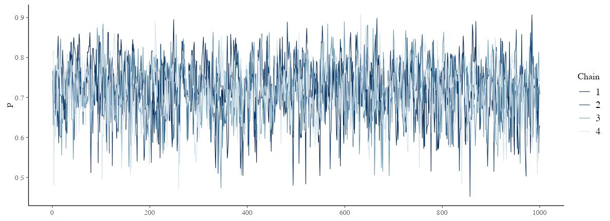
念のため trace plot も確認しておこう→

説明変数なしのベイズ推定: trace plot 確認

どのchainも似た範囲を動いていて、しっかり毛虫っぽい:

draws = fit$draws()
params = names(model$variables()$parameters)
bayesplot::mcmc_trace(draws, pars = params)

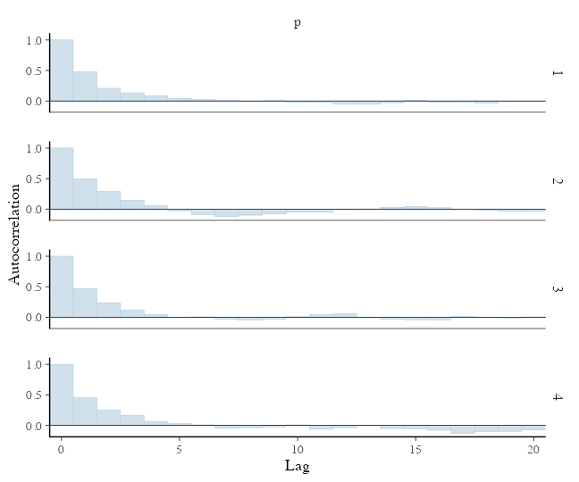
説明変数なしのベイズ推定: 自己相関の確認

2–3ステップくらいで自己相関がほぼ消えるので問題なし:

bayesplot::mcmc_acf_bar(draws, pars = params)

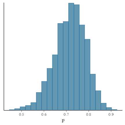
説明変数なしのベイズ推定: 推定結果確認

サンプルサイズNが小さいせいか裾野の広い推定結果。
真の$p$の値も含まれている:

bayesplot::mcmc_hist(draws, bins = 20, pars = params)

lp__: log posterior とは?

model ブロックに次のように書いてあると:

model {
  mu ~ normal(0.0, 10.0);  // prior
  x ~ normal(mu, 1.0);     // likelihood
}

内部的には次のような処理が行われている:

target += normal_lpdf(theta | 0.0, 10.0)  // prior
target += normal_lpdf(x | theta, 1.0);    // likelihood

つまり、事前確率と尤度の対数の和を取っている。
ベイズの定理により、事後確率はこれに比例する。
lp__ はこの target 変数を記録しておいたようなもの。

Stanで回帰じゃないパラメータ推定、まとめ

別ファイルに書いておく。 e.g., coin.stan:

data {
  int<lower=0> N;
  array[N] int x;
}
parameters {
  real<lower=0,upper=1> p;
}
model {
  x ~ binomial(1, p);
}

Rからデータを渡して走らせる:

coin_data = tibble::lst(N = 50L, x = rbinom(N, 1, 0.7))
coin_model = cmdstanr::cmdstan_model("stan/binom.stan")
coin_fit = coin_model$sample(coin_data, seed = 24601L)

直線回帰するStanコードの例

受け渡しするデータや推定するパラメータがちょっと増えただけ。

data {
  int<lower=0> N;
  vector<lower=0>[N] x;
  vector[N] y;
}

parameters {
  real intercept;
  real slope;
  real<lower=0> sigma;
}

model {
  y ~ normal(intercept + slope * x, sigma);
}

Rと同様、 slope * x のようなベクトル演算ができる。

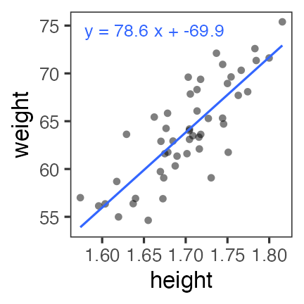
直線回帰っぽいデータに当てはめてみる

sample_size = 50L
df_lm = tibble::tibble(
  x = rnorm(sample_size, 1.70, 0.05),
  bmi = rnorm(sample_size, 22, 1),
  y = bmi * (x**2)
)

操作は回帰じゃないモデルと同じ

# リストに入れて渡す:
lm_data = as.list(df_lm)
lm_data[["N"]] = sample_size
# モデルを実行速度の速い機械語に翻訳(コンパイル):
lm_model = cmdstanr::cmdstan_model("stan/lm.stan")
# モデルとデータを使ってMCMCサンプリング:
lm_fit = lm_model$sample(lm_data, seed = 19937L, refresh = 0)

print(lm_fit)

  variable   mean median    sd   mad     q5    q95 rhat ess_bulk ess_tail
 lp__      -79.49 -79.16  1.30  1.07 -82.06 -78.08 1.00     1065     1341
 intercept -68.54 -69.16 14.57 14.59 -91.28 -43.45 1.00      886      777
 slope      77.87  78.18  8.56  8.58  63.13  91.30 1.00      887      797
 sigma       3.08   3.04  0.33  0.32   2.62   3.65 1.00     1381     1340

切片と傾きはそれらしき値。 $\hat R$ や $N_{eff}$ も良さそう。 もう少し確認しよう。

CmdStanによる診断

lm_fit$cmdstan_diagnose()

satisfactory とか no problems ばかりであることを確認

Treedepth satisfactory for all transitions.

No divergent transitions found.

E-BFMI satisfactory.

Effective sample size satisfactory.

Split R-hat values satisfactory all parameters.

Processing complete, no problems detected.

draws: 生のMCMCサンプル

lm_draws_array = lm_fit$draws()
dim(lm_draws_array)

[1] 1000    4    4

print(lm_draws_array)

# A draws_array: 1000 iterations, 4 chains, and 4 variables
, , variable = lp__

         chain
iteration   1   2   3   4
        1 -79 -79 -78 -82
        2 -79 -80 -78 -81
        3 -78 -78 -79 -82
        4 -78 -78 -79 -82
        5 -81 -78 -79 -80

, , variable = intercept

         chain
iteration   1   2   3   4
        1 -53 -74 -71 -34
        2 -58 -74 -76 -38
        3 -65 -74 -62 -36
        4 -72 -72 -58 -39
        5 -90 -62 -58 -65

, , variable = slope

         chain
iteration  1  2  3  4
        1 68 81 79 57
        2 72 81 82 60
        3 76 81 74 59
        4 80 80 72 61
        5 90 74 72 76

, , variable = sigma

         chain
iteration   1   2   3   4
        1 3.2 2.7 3.1 3.5
        2 2.8 2.7 2.9 2.9
        3 2.9 2.7 2.8 2.9
        4 3.2 2.7 2.8 3.5
        5 3.7 3.0 2.8 2.6

# ... with 995 more iterations

draws: data.frameのほうが見やすいかも

lm_draws = lm_fit$draws(format = "df") |> print()

# A draws_df: 1000 iterations, 4 chains, and 4 variables
   lp__ intercept slope sigma
1   -79       -53    68   3.2
2   -79       -58    72   2.8
3   -78       -65    76   2.9
4   -78       -72    80   3.2
5   -81       -90    90   3.7
6   -80       -85    88   3.4
7   -79       -86    88   3.1
8   -79       -85    87   3.0
9   -79       -64    75   2.6
10  -79       -63    74   3.4
# ... with 3990 more draws
# ... hidden reserved variables {'.chain', '.iteration', '.draw'}

実体はCmdStanが書き出したCSVファイル:

lm_fit$output_files()

[1] "/var/folders/**/***/T/Rtmp******/*-2023****-1-******.csv"
[2] "/var/folders/**/***/T/Rtmp******/*-2023****-2-******.csv"
[3] "/var/folders/**/***/T/Rtmp******/*-2023****-3-******.csv"
[4] "/var/folders/**/***/T/Rtmp******/*-2023****-4-******.csv"

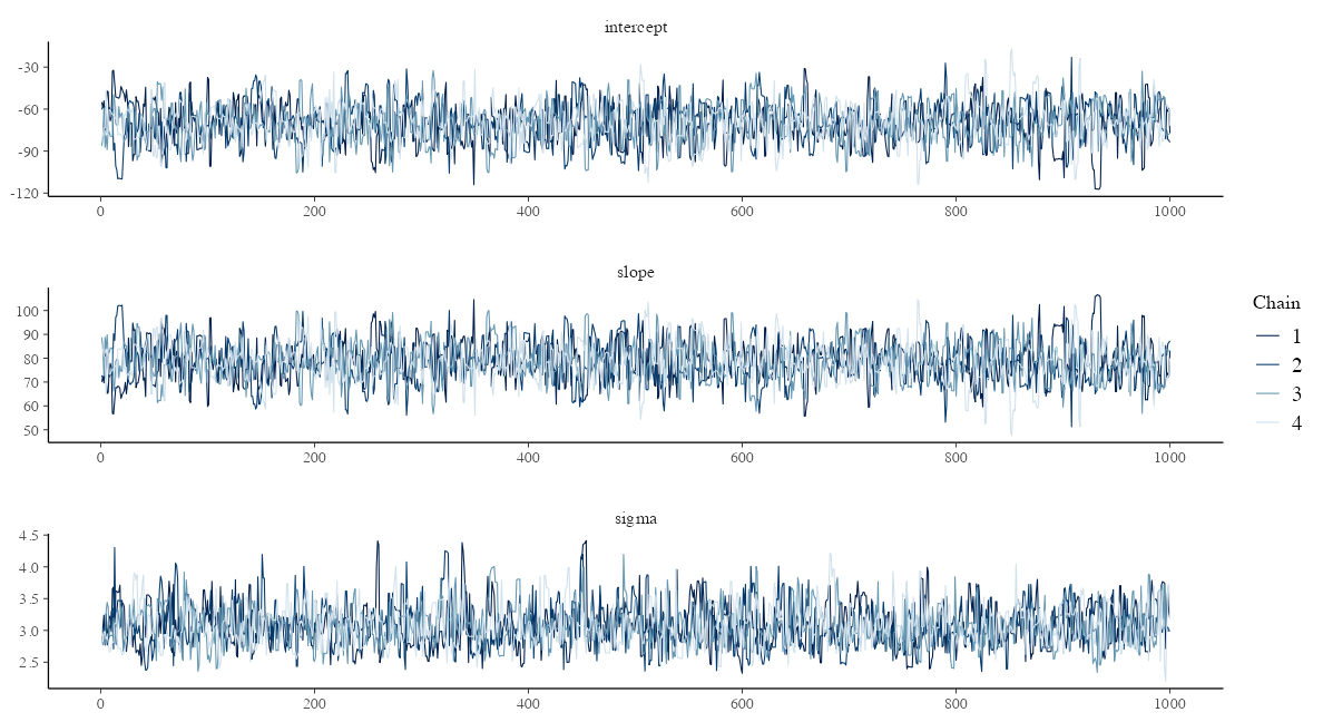
traceplot: サンプル順に draws を並べたもの

どの chain も同じところをうろうろしていればOK。

params = names(lm_model$variables()$parameters)
bayesplot::mcmc_trace(lm_draws, pars = params, facet_args = list(ncol = 1))

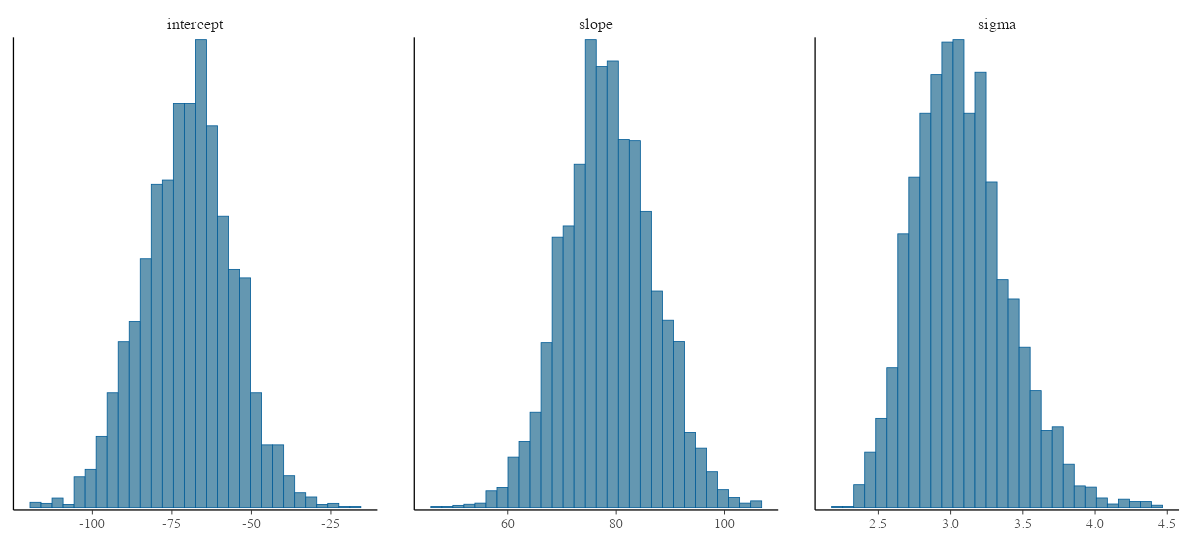
各パラメータの事後分布

bayesplot::mcmc_hist(lm_draws, pars = params, bins = 30)

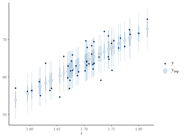
Posterior Predictive Checking (PPC)

サイズ $S$ のパラメータdrawsと $N$ 個の観察値から $S \times N$ 行列の $y_{rep}$ を生成:

mu_rep = lm_draws$intercept + lm_draws$slope %o% df_lm$x
yrep = mu_rep + rnorm(prod(dim(mu_rep)), 0, lm_draws$sigma)
bayesplot::ppc_intervals(y = df_lm[["y"]], yrep = yrep,
  x = df_lm[["x"]], prob = 0.5, prob_outer = 0.9)

http://mc-stan.org/bayesplot/reference/PPC-overview.html

変数とブロックをうまく使って可読性アップ

途中計算に名前をつけることでモデルが読みやすくなる:

model {
  vector[N] mu = intercept + slope * x;
  y ~ normal(mu, sigma);
}

transformed parameters ブロックに書くとさらに見通しがよくなる:

transformed parameters {
  vector[N] mu = intercept + slope * x;
}

model {
  y ~ normal(mu, sigma);
}

見た目が変わるだけでなくMCMCサンプルが記録されるようになる。

drawsは嵩むが頭は使わずに済む

lmtr_model = cmdstanr::cmdstan_model("stan/lm-transformed.stan")
lmtr_fit = lmtr_model$sample(lm_data, seed = 19937L, refresh = 0)
lmtr_draws = lmtr_fit$draws(format = "df") |> print()

# A draws_df: 1000 iterations, 4 chains, and 54 variables
   lp__ intercept slope sigma mu[1] mu[2] mu[3] mu[4] mu[5] mu[6] mu[7] mu[8] mu[9] mu[10] mu[11] mu[12] mu[13] mu[14] mu[15] mu[16] mu[17] mu[18] mu[19] mu[20] mu[21] mu[22] mu[23] mu[24] mu[25] mu[26] mu[27] mu[28] mu[29] mu[30] mu[31] mu[32] mu[33] mu[34] mu[35] mu[36] mu[37] mu[38] mu[39] mu[40] mu[41] mu[42] mu[43] mu[44] mu[45] mu[46] mu[47] mu[48] mu[49] mu[50]
1 -79.1     -52.6  68.3  3.25  64.8  69.2  57.9  62.1  64.7  58.7  69.3  61.8  59.3   63.9   67.3   62.5   61.5   64.7   62.9   62.7   66.7   61.5   58.1   57.0   61.7   63.9   64.8   66.1   63.9   61.9   63.7   59.5   70.4   63.8   71.5   67.0   64.5   63.9   68.1   66.6   56.4   65.4   68.6   54.9   64.5   67.0   61.0   62.1   60.5   64.2   67.9   66.6   65.7   62.0
2 -78.6     -58.4  71.8  2.80  64.9  69.6  57.7  62.1  64.8  58.6  69.7  61.8  59.1   64.0   67.5   62.6   61.5   64.8   62.9   62.7   66.9   61.5   57.9   56.7   61.7   64.0   64.9   66.3   64.0   61.8   63.8   59.3   70.8   63.9   71.9   67.3   64.6   64.0   68.4   66.8   56.2   65.6   69.0   54.6   64.6   67.2   60.9   62.1   60.4   64.3   68.2   66.8   65.8   62.0
3 -78.1     -64.5  75.6  2.91  65.4  70.3  57.8  62.4  65.2  58.7  70.4  62.0  59.3   64.4   68.1   62.9   61.7   65.3   63.2   63.1   67.5   61.8   57.9   56.7   62.0   64.4   65.4   66.8   64.4   62.1   64.1   59.5   71.6   64.3   72.8   67.9   65.1   64.4   69.0   67.4   56.1   66.1   69.6   54.5   65.0   67.8   61.2   62.4   60.6   64.7   68.8   67.4   66.3   62.2
4 -78.5     -72.4  80.3  3.20  65.6  70.8  57.6  62.4  65.5  58.5  71.0  62.1  59.1   64.6   68.5   63.0   61.7   65.5   63.3   63.2   67.8   61.8   57.7   56.4   62.0   64.5   65.6   67.1   64.5   62.2   64.3   59.4   72.2   64.4   73.5   68.3   65.3   64.5   69.5   67.7   55.8   66.4   70.1   54.0   65.3   68.2   61.2   62.5   60.6   64.9   69.2   67.7   66.6   62.3
5 -81.0     -89.7  90.0  3.72  65.0  70.8  56.0  61.4  64.8  57.0  71.0  61.0  57.7   63.9   68.3   62.0   60.7   64.9   62.5   62.3   67.5   60.7   56.1   54.7   60.9   63.8   65.0   66.7   63.8   61.1   63.5   58.0   72.4   63.7   73.8   68.0   64.6   63.8   69.4   67.4   54.0   65.8   70.1   52.0   64.6   67.9   60.0   61.5   59.3   64.2   69.1   67.4   66.1   61.3
6 -79.6     -84.7  87.6  3.40  65.8  71.5  57.0  62.3  65.6  58.0  71.6  61.9  58.7   64.7   69.0   62.9   61.6   65.7   63.3   63.1   68.2   61.7   57.2   55.8   61.9   64.6   65.8   67.5   64.6   62.1   64.4   59.0   73.0   64.5   74.4   68.7   65.4   64.6   70.1   68.1   55.1   66.6   70.7   53.2   65.4   68.6   60.9   62.4   60.3   65.0   69.8   68.1   66.9   62.2
# ... with 3994 more draws
# ... hidden reserved variables {'.chain', '.iteration', '.draw'}

この右側の mu 行列はさっき苦労して作った mu_rep と同じ。

ひょっとして yrep もStanで作れる？

generated quantities ブロックで乱数生成

(data と parameters のブロックは同じなので省略)

transformed parameters {
  vector[N] mu = intercept + slope * x;
}

model {
  y ~ normal(mu, sigma);
}

generated quantities {
  array[N] real yrep = normal_rng(mu, sigma);
}

normal_rng() のような乱数生成が使えるのは
generated quantities ブロックだけ。

(yrep を vector[N] 型で作ろうとすると怒られる。)

drawsはさらに嵩むがコードは美しくなった

lmgen_model = cmdstanr::cmdstan_model("stan/lm-generated.stan")
lmgen_fit = lmgen_model$sample(lm_data, seed = 19937L, refresh = 0)
lmgen_draws = lmgen_fit$draws(format = "df") |> print()

# A draws_df: 1000 iterations, 4 chains, and 104 variables
   lp__ intercept slope sigma mu[1] mu[2] mu[3] mu[4] mu[5] mu[6] mu[7] mu[8] mu[9] mu[10] mu[11] mu[12] mu[13] mu[14] mu[15] mu[16] mu[17] mu[18] mu[19] mu[20] mu[21] mu[22] mu[23] mu[24] mu[25] mu[26] mu[27] mu[28] mu[29] mu[30] mu[31] mu[32] mu[33] mu[34] mu[35] mu[36] mu[37] mu[38] mu[39] mu[40] mu[41] mu[42] mu[43] mu[44] mu[45] mu[46] mu[47] mu[48] mu[49] mu[50] yrep[1] yrep[2] yrep[3] yrep[4] yrep[5] yrep[6] yrep[7] yrep[8] yrep[9] yrep[10] yrep[11] yrep[12] yrep[13] yrep[14] yrep[15] yrep[16] yrep[17] yrep[18] yrep[19] yrep[20] yrep[21] yrep[22] yrep[23] yrep[24] yrep[25] yrep[26] yrep[27] yrep[28] yrep[29] yrep[30] yrep[31] yrep[32] yrep[33] yrep[34] yrep[35] yrep[36] yrep[37] yrep[38] yrep[39] yrep[40] yrep[41] yrep[42] yrep[43] yrep[44] yrep[45] yrep[46] yrep[47] yrep[48] yrep[49] yrep[50]
1 -79.1     -52.6  68.3  3.25  64.8  69.2  57.9  62.1  64.7  58.7  69.3  61.8  59.3   63.9   67.3   62.5   61.5   64.7   62.9   62.7   66.7   61.5   58.1   57.0   61.7   63.9   64.8   66.1   63.9   61.9   63.7   59.5   70.4   63.8   71.5   67.0   64.5   63.9   68.1   66.6   56.4   65.4   68.6   54.9   64.5   67.0   61.0   62.1   60.5   64.2   67.9   66.6   65.7   62.0    63.7    70.2    60.3    65.1    68.6    55.8    71.9    58.7    59.3     62.6     66.6     63.4     62.8     65.1     61.4     59.7     68.9     60.9     57.3     55.2     62.0     61.5     73.5     74.5     66.2     61.8     67.0     54.7     72.3     63.1     69.9     74.7     62.9     65.7     71.1     68.2     53.4     71.4     67.1     51.9     63.8     67.9     63.0     57.6     64.0     63.0     65.1     66.6     61.9     61.8
2 -80.1     -46.0  64.3  3.10  64.5  68.7  58.1  62.0  64.4  58.8  68.8  61.7  59.3   63.7   66.9   62.4   61.4   64.4   62.7   62.6   66.3   61.5   58.2   57.2   61.6   63.7   64.5   65.7   63.7   61.8   63.5   59.5   69.8   63.6   70.8   66.7   64.3   63.7   67.7   66.2   56.7   65.1   68.1   55.3   64.2   66.6   61.0   62.0   60.5   63.9   67.4   66.2   65.3   61.9    62.4    70.7    57.1    58.7    71.2    56.6    70.2    61.9    57.0     65.6     70.0     63.5     60.5     60.1     65.3     62.3     70.1     64.9     58.2     56.1     59.3     60.9     64.2     64.3     64.2     62.4     65.3     54.8     70.9     60.6     68.9     70.9     65.6     64.8     68.9     66.5     57.3     64.4     69.5     55.8     64.5     71.4     64.4     63.6     63.8     69.0     70.2     64.8     67.1     61.5
3 -79.6     -46.3  64.9  3.07  65.3  69.5  58.8  62.7  65.2  59.5  69.6  62.4  60.0   64.5   67.7   63.1   62.2   65.2   63.5   63.3   67.1   62.2   58.9   57.9   62.4   64.4   65.3   66.5   64.4   62.5   64.2   60.2   70.6   64.3   71.6   67.4   65.0   64.4   68.4   67.0   57.4   65.9   69.0   55.9   65.0   67.4   61.7   62.7   61.2   64.7   68.2   67.0   66.1   62.6    64.4    70.6    60.9    66.8    66.5    57.6    72.4    61.6    59.6     63.8     75.2     67.1     58.6     64.2     65.1     68.0     70.2     63.2     56.2     50.7     61.6     63.4     63.7     67.5     63.4     66.6     69.0     61.5     78.4     67.4     71.0     74.4     64.7     62.8     65.0     66.6     56.2     66.2     71.7     55.2     58.9     70.1     65.5     64.7     60.1     65.2     69.3     72.8     60.8     62.8
4 -78.9     -51.4  67.8  2.98  65.2  69.6  58.3  62.5  65.0  59.1  69.7  62.2  59.7   64.3   67.6   62.9   61.9   65.0   63.2   63.1   67.0   61.9   58.5   57.4   62.1   64.2   65.1   66.4   64.2   62.2   64.0   59.9   70.7   64.1   71.8   67.4   64.9   64.2   68.4   66.9   56.9   65.8   69.0   55.4   64.9   67.3   61.4   62.5   60.9   64.5   68.2   66.9   66.0   62.3    62.7    70.1    55.7    60.4    71.1    62.1    74.3    61.9    57.7     65.0     72.5     67.3     66.1     70.3     66.1     64.1     71.4     58.3     58.5     55.7     64.8     67.7     65.6     66.0     67.0     62.4     60.5     58.5     67.9     61.3     76.9     68.4     60.0     63.6     68.9     67.2     54.2     64.2     71.8     58.7     69.8     67.9     58.5     62.6     61.2     66.3     63.5     73.6     66.5     62.7
5 -78.7     -53.6  69.2  3.07  65.3  69.8  58.3  62.6  65.2  59.2  69.9  62.2  59.7   64.4   67.8   63.0   62.0   65.2   63.3   63.2   67.2   62.0   58.5   57.4   62.2   64.4   65.3   66.6   64.4   62.3   64.2   59.9   71.0   64.3   72.1   67.6   65.0   64.4   68.7   67.1   56.8   65.9   69.2   55.3   65.0   67.5   61.5   62.6   60.9   64.7   68.4   67.1   66.2   62.4    68.2    65.9    62.6    64.4    63.9    57.3    70.4    55.7    54.6     62.6     65.0     63.3     61.6     69.4     63.5     64.4     69.9     62.2     58.9     57.6     54.9     64.0     60.9     62.3     65.6     64.0     60.8     60.0     67.8     62.9     72.5     66.6     57.6     60.5     69.6     70.4     56.2     66.5     65.5     53.8     65.5     70.4     62.4     59.9     52.9     63.1     63.4     67.2     66.5     57.3
6 -79.3     -87.7  88.9  3.20  65.0  70.8  56.1  61.5  64.8  57.1  70.9  61.1  57.8   63.9   68.2   62.1   60.7   64.9   62.5   62.3   67.4   60.8   56.3   54.8   61.0   63.8   65.0   66.7   63.8   61.2   63.5   58.1   72.3   63.7   73.7   67.9   64.6   63.8   69.3   67.3   54.1   65.8   70.0   52.2   64.6   67.8   60.1   61.5   59.4   64.2   69.0   67.3   66.1   61.3    61.6    71.3    53.2    61.4    65.5    54.7    67.7    63.4    53.5     67.1     71.4     64.6     57.9     63.0     62.9     57.2     64.8     55.2     53.2     57.6     62.9     55.3     61.4     63.7     64.5     58.9     64.0     58.4     71.0     63.9     71.5     70.2     64.8     63.1     73.5     61.0     60.5     65.7     62.9     51.0     65.3     74.5     54.9     59.7     65.2     61.2     61.8     64.2     65.4     61.0
# ... with 3994 more draws
# ... hidden reserved variables {'.chain', '.iteration', '.draw'}

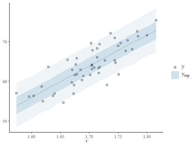
yrep = lmgen_fit$draws("yrep", format = "matrix") を取り出したらあとは bayesplot::ppc_*() に渡すだけ。

観察値とは違うXを使ってPredictionすることも可能

観察値の外側とか、均等間隔とか x_tilde を好きに作って渡せる。

data {
  // ...
  int<lower=0> N_tilde
  vector[N_tilde] x_tilde;
}
// ...
generated quantities {
  array[N_tilde] real y_tilde = normal_rng(intercept + slope * x_tilde, sigma);
}

変数の型: vector vs array

vector, row_vector, matrix は実数 real のみで、行列演算できる:

real x;
vector[3] v;
row_vector[3] r;
matrix[3, 3] m;

x * v  // vector[3]
r * v  // real
v * r  // matrix[3, 3]
m * v  // vector[3]
m * m  // matrix[3, 3]
m[1]   // row_vector[3]

array に型の制約は無いが、行列演算はできないので自力forループ:

array[3] int a;
array[3] int b;
for (i in 1:3) {
  b[i] = 2 * a[i] + 1
}

パラメータの事前分布を明示的に設定できる

が、省略してもStanがデフォルトでうまくやってくれる。
そのせいで収束が悪いかも、となってから考えても遅くない。

parameters {
  real intercept;
  real slope;
  real<lower=0> sigma;
}

model {
  y ~ normal(intercept + slope * x, sigma);
  intercept ~ normal(0, 100);
  slope ~ normal(0, 100);
  sigma ~ student_t(3, 0, 10);
}

設定したくなったら、どう選ぶか？

事前分布の選別

1. とりあえず無情報事前分布 $[-\infty, \infty]$。Stanのデフォルト。

2. 収束が悪かったら弱情報事前分布を試す。
   事後分布を更新していったとき事前分布っぽさが残らないのが良い。

   • 取りうる値を逃すような狭すぎる分布はダメ。
   • 狭すぎるよりはマシだが、広すぎても良くない。
   • 一様分布 $[a, b]$ は一見無情報っぽくて良さそうだが、
     事後分布に裾野が残ったり絶壁ができたりしがちなので微妙。

   おすすめ: 正規分布 or Student’s t分布

https://github.com/stan-dev/stan/wiki/Prior-Choice-Recommendations

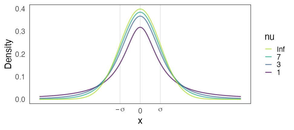
Stanおすすめ弱情報事前分布: Student’s t分布

Student’s $t(\nu=\nu_0, \mu = 0, \sigma = \sigma_0)$

• 自由度 $3 \le \nu_0 \le 7 $ で適当に固定。
  • $\nu = 1$ でコーシー分布。裾野が広すぎて良くないらしい。
  • $\nu \to \infty$ で正規分布。だいたいこれでいいらしい。
• スケール $\sigma$: 「推定したい値は$[-\sigma_0, \sigma_0]$に収まるだろう」という値。

🔰 Stanで一般化線形モデル

🔰 7-stan.ipynb を開いて実行していこう。

• 直線回帰

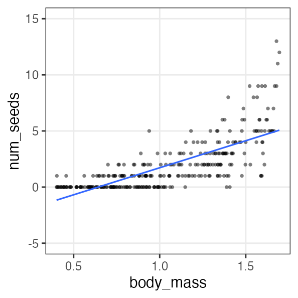
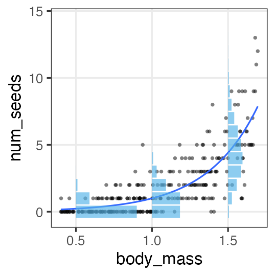
• ポアソン回帰

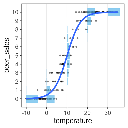
• ロジスティック回帰

• 重回帰

• 分散分析

• 共分散分析

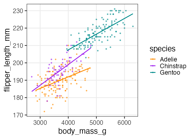
🔰 Stanでpenguinsの回帰分析をしてみよう

https://allisonhorst.github.io/palmerpenguins/

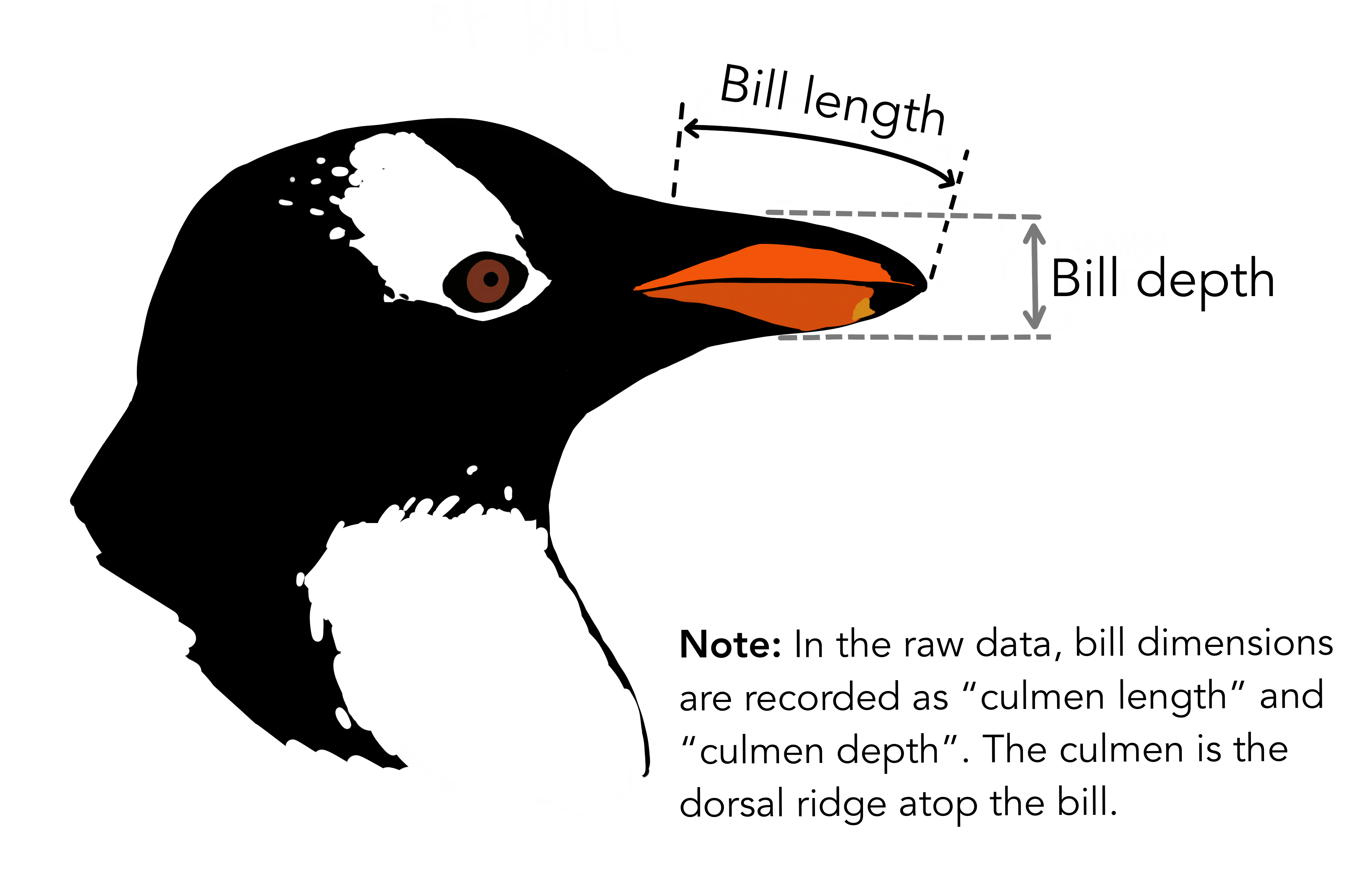
GLM回の練習を参照。

🔰 Stanでpenguinsの回帰分析をしてみよう

https://allisonhorst.github.io/palmerpenguins/

Stan does not support NA と怒られるので欠損値を取り除いておく:

penguins = sm.datasets.get_rdataset("penguins", "palmerpenguins", True).data
penguins_dropna = penguins.dropna()

参考文献

• データ解析のための統計モデリング入門 久保拓弥 2012
• StanとRでベイズ統計モデリング 松浦健太郎 2016
• RとStanではじめる ベイズ統計モデリングによるデータ分析入門 馬場真哉 2019
• データ分析のための数理モデル入門 江崎貴裕 2020
• 分析者のためのデータ解釈学入門 江崎貴裕 2020
• 統計学を哲学する 大塚淳 2020